
The analytic hierarchy process with personalized individual semantics
- DOI
- 10.2991/ijcis.11.1.34How to use a DOI?
- Keywords
- Analytic hierarchy process (AHP); personalized individual semantics (PIS); numerical scale; the 2-tuple linguistic model; consistency-driven methodology
- Abstract
Personalized individual semantics (PIS) is not unusual in our daily life, and it has an important influence on the final decision results in linguistic decision making. The analytic hierarchy process (AHP) has now become a popular decision tool because of its sound mathematical design and ease of applicability to real-world decision making problems. In the AHP, two formats of preference information are included: linguistic and numerical preference information. In order to implement the computation operation, the linguistic preference information is often transformed into the numerical preference information using a fixed numerical scale function (e.g., the Saaty scale). However, the PIS is not taken into account by the AHP with a fixed numerical scale function. Therefore, this study proposes a novel AHP framework with the PIS, and develops a consistency-driven methodology to minimize the inconsistency level of numerical preference information that transformed from linguistic preference information. In the proposed AHP framework, a two-stage based optimization model is designed to deal with the PIS, and the proposed optimization models are converted into some linear programming models that can be easily solved. Finally, a practical example and a comparison experiment are proposed to verify the validity of our proposal.
- Copyright
- © 2018, the Authors. Published by Atlantis Press.
- Open Access
- This is an open access article under the CC BY-NC license (http://creativecommons.org/licences/by-nc/4.0/).
1. Introduction
The analytic hierarchy process (AHP) that initialized by Saaty (1980) provides decision makers with a way to transform subjective judgments into objective measures[38]. Due to its mathematical simplicity and flexibility, AHP has been a favorite decision tool for research in many fields [43], such as manufacture, politics and economy, power and energy, education, and medicine. In general, the implementation of the AHP includes the following steps: (1) construct a decision-making problem in a hierarchy as goal, criteria, sub-criteria, and decision alternatives; (2) provide linguistic preference information (i.e., linguistic pairwise comparison matrices (LPCMs), or linguistic preference relations) at each level of the hierarchy structure; (3) transform the linguistic preference information into numerical preference information (i.e., numerical pairwise comparison matrices (NPCMs)) using a numerical scale function (i.e., the Saaty scale); (4) check the consistency of numerical preference information; (5) obtain the local priority vectors corresponding to the criteria or sub-criteria applying the given prioritization method (e.g., Eigenvalue method); (6) obtain the global priority vectors of alternatives by synthesizing the local priority vectors. The detailed information of the AHP can be found in [13, 38, 40].
By analyzing the implementation process of the AHP, we find that the validity of which depends on the selection of numerical scale function in step 3. This issue has been investigated by several scholars, and several numerical scale functions have been proposed, such as the Saaty scale function [38], the Ma-Zheng scale function [30], the geometrical scale function [21, 26, 29], and the Salo Hämäläinen scale function [37]. However, there are still some disputes on which numerical scale function is better. Harker and Vargas [23] argued that the choice of numerical scale function in the AHP is an open problem.
The selection of numerical scale in the AHP is closely related to the computing with words (CWW). In the field of CWW, there is a fact that the same word usually means different things for different experts ([31, 32]). For example, two experts may all provide their comments “good” on a project in the project review process. However, the term “good” often refers to different scores for these two experts when they grade the project on a scale of 0 to 100, one expert might give 80 and another give 90. There are two mainstreams in the literature to deal with this issue: (1) the type-2 fuzzy sets [31], (2) the multi-granular linguistic models [16, 34, 45, 50]. Despite these approaches are quite useful, they do not present the specific semantics for each expert. To overcome this problem, Li et al. [27] proposed an optimization-based model to deal with personalized individual semantics (PIS for short) in the linguistic decision making.
Based on the above analysis, there is no doubt that the PIS will occur in the AHP, and it has a very important influence on the final decision results. To our knowledge, the PIS is rarely considered by the existing literature except two works [25, 35]. In [25, 35], the existence of PIS in the AHP has been demonstrated by using empirical study. However, an effective way to deal with the PIS in the AHP is not provided in [25, 35].
The main purpose of this study is to propose a novel AHP framework: the AHP framework with the PIS. In the novel AHP, the most important step is the design of the transformation method between the linguistic and numerical preference information. To support the novel framework, we devise a consistency-driven approach that minimizes the consistency index of the transformed numerical preference information. This approach is based on a basic idea that if linguistic preference information is of acceptable consistency, then the consistency level of the transformed numerical preference information should be as better as possible, due to the fact that both the linguistic and numerical preference information are associated with the same expert. Specifically, we propose a two-stage based optimization model to address the PIS in the AHP. The first-stage optimization model is used to generate the individual numerical scales by maximizing the consistency level of the transformed numerical preference information, and the second-stage optimization model is utilized to further optimize the optimal solutions derived from the first-stage model. In addition, both the optimization models in first and second stages are converted into linear programming models that can be easily solved.
The remainder of this study is arranged as follows. Section 2 introduces the 2-tuple linguistic model, numerical scales and the AHP with a fixed numerical scale function. Section 3 designs a novel AHP framework with the PIS. Next, Section 4 presents the consistency-driven approach to deal with the PIS in the AHP. Following this, a practical example is used to illustrate the application process of our proposal. Section 6 gives a comparative study. Finally, Section 7 concludes the study and discusses the future research directions.
2. Preliminaries
In this section, the fundamental knowledge regarding the 2-tuple linguistic model, preference relations, numerical scales, and the AHP with a fixed numerical scale, are briefly described.
2.1. The 2-tuple linguistic model and preference relations
(1) The 2-tuple linguistic model
Let S= {si|i = 0,1,2,...,g} be a linguistic term set, in which the number of linguistic terms is odd (i.e., g+1). The term si denotes a possible value for a linguistic variable, and the following two conditions should be satisfied [15].
- (i)
If i > j, then si > sj.
- (ii)
We have Neg (si) = sj such that j = g – i, where Neg denotes a negation operator.
The 2-tuple linguistic model that proposed by Herrera and Martínez [24] is a popular model for computing with words. Let S be as above. In the 2-tuple linguistic model, a 2-tuple (si, α) is utilized to express the equivalent information to β ∈ [0, g]: Δ :[0, g] → S × [−0.5, 0.5), where
(2) Preference relations
Let X = {x1, x2,...,xn} be a set of alternatives. During the decision making process, preference relations (e.g. [7, 28, 22]) are very useful tools for decision makers to express their preferences over X. In particular, linguistic and multiplicative preference relations are widely adopted in the decision making. In the following, we introduce these two types of preference relations.
Definition 1 [1, 12]:
The linguistic preference relation is represented by a matrix L = (lij)n×n, in which the element lij ∈ S signifies the preference intensity of alternative xi over xj. The linguistic preference relation L = (lij)n×n is often assumed to be reciprocal, that is lij = Neg(lji) for i, j = 1,...,n.
Definition 2 [40, 46]:
The multiplicative preference relation is denoted using a matrix A = (aij)n×n, in which aij > 0 signifies the important degree (or preference intensity) of alternative xi over xj and aij × aji = 1 for i, j = 1,….,n. If ait × atj = aij (∀ i, j, t = 1,2,...,n), then A is considered as a completely consistent multiplicative preference relation.
2.2. Numerical scales
The numerical scale was developed by Dong et al. [19], which is utilized to convert linguistic information into numerical information.
Definition 3 [19]:
Let S be as before, and R be the real number set. The numerical scale of S is defined as a function: NS : S → R, and we use NS(si) to denote the numerical index of linguistic term is si.
Moreover, the numerical scale of the 2-tuple linguistic information was also developed, which is defined as follows.
Definition 4 [19]:
Let S,
For simplification,
2.3. Analytic hierarchy process
This section introduces the basic framework of AHP, and the 2-tuple linguistic modeling for the AHP scale problem.
(1) The framework of AHP
Saaty [38] developed following steps for applying the AHP.
a) Establish the hierarchical structure
When using AHP to solve a decision problem, firstly, decision makers need to disassemble the problem into a hierarchy of more easily comprehended sub-problems. A hierarchical structure (shown as Fig. 1) is often composed by the following levels: goal level, criterion levels, and alternative level. In addition, there are subordinate relationships between the elements on two adjacent levels in the hierarchy.
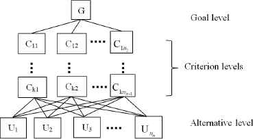
The hierarchical structure.
Let Hk (k = 1,...,m) be the k th level of the given hierarchical structure. The top level (i.e., H1) is the goal level, the bottom level (i.e., Hm) is the alternative level, the others are criterion levels. Let nk (k = 1,...,m) be the number of elements (criteria/alternatives) in Hk. In particular, nm denotes the number of alternatives. Let
b) Make pairwise comparisons using AHP linguistic scale to obtain linguistic preference relations
Decision makers provide their linguistic preference information regarding criteria and alternatives corresponding to the parent element at the adjacent upper level. For the parent element
c) Transform LPCMs into NPCMs using AHP numerical scale
In the traditional AHP, decision makers employ a fixed numerical scale (i.e., the Saaty scale) to transform the LPCMs
d) Employ a prioritization method to derive the local priority vectors of criteria and alternatives
By adopting a selected prioritization method, we can derive priority vectors
To derive a priority vector from a NPCM A = (aij)n× n, the prioritization method is often used. There are several prioritization methods (e.g., [8, 9, 33, 38, 39, 41, 49]). In this paper, we adopt the Eigenvalue method proposed by Saaty [39], which is introduced below.
Let λ and p′ be the eigenvalue and eigenvector of matrix A, respectively, and they can be obtained by the following model:
Saaty sets the principle eigenvector as the desired priority vector of A.
e) Consistency test
Consistency test is adopted to check whether the NPCMs are logical or not. If the NPCMs fail the consistency test, decision maker should adjust the corresponding LPCMs. There are many consistency improving approaches [5, 47]. In particular, the consistency index (CI) based on the eigenvalue prioritization method proposed by Saaty [38] is calculated as below:
Further, Saaty proposed the concept of consistency ratio, that is
| n | 3 | 4 | 5 | 6 | 7 | 8 | 9 |
|---|---|---|---|---|---|---|---|
| RI | 0.52 | 0.89 | 1.12 | 1.26 | 1.36 | 1.41 | 1.46 |
Values of RI for different matrix size (n)
In addition, there are several other approaches for measuring the consistency level of NPCMs (see [2, 3, 6, 14, 42]).
f) Synthesize the priority vectors to yield the global priority vector
This process is to synthesize the local priority vectors with respect to all criteria to generate the global priority vectors. Further, we can obtain the ranking of the alternatives from the global priority vector at the alternative level.
Suppose that
Therefore, wk = PkPk−1 … w2 and
(2) 2-tuple linguistic modeling of the AHP scale problem
The scale in AHP is composed of AHP linguistic and numerical scales. Table 2 shows the Saaty’s linguistic scale (see [40]).
| Grade | AHP linguistic scale |
|---|---|
| 1 | Equally important |
| 2 | Weakly more important |
| 3 | Moderately more important |
| 4 | Moderately plus more important |
| 5 | Strongly more important |
| 6 | Strongly more important |
| 7 | Demonstratedly more important |
| 8 | Very, very Strongly more important |
| 9 | Extremely more important |
Linguistic part of the Saaty scale
According to Saaty’s linguistic scale, we define the following linguistic term set [12]:
SAHP = {s0 = extremely less important, s1 = very very strongly less important, s2 = demonstratedly less important, s3 = strongly plus less important, s4 = strongly less important, s5 = moderately plus less important, s6 = moderately less important, s7 = weakly less important, s8 = equally important, s9 = weakly more important, s10 = moderately more important, s11 = moderately plus more important, s12 = strongly more important, s13 = strongly plus more important, s14 = demonstratedly more important, s15 = very very strongly more important, s16 = extremely more important}
There are 17 numerical values in the AHP numerical scale, which are described below:
In [13], based on the 2-tuple linguistic model, the AHP numerical scale is developed, which is defined as below:
Definition 5 [13]:
Let
Based on the AHP numerical scale function, we can transform an LPCM L = (lij)n×n into a NPCM A = (aij)n×n, where aij = NSAHP (lij) for i, j = 1, 2, …..,n.
3. The framework of the AHP with PIS
By taking into account an un-negligible factor, PIS, in the AHP, this section proposes a novel AHP framework: the AHP framework with PIS.
As introduced in Section 2, in the traditional AHP, a decision maker provides LPCMs in the established hierarchical structure. Then, for conducting computation operation, LPCMs are transformed into NPCMs using a certain numerical scale function. The choice of numerical scale has an important influence on the final decision results, and there are several common numerical scale functions (e.g., [21, 26, 29, 30, 37, 38]). When selecting a numerical scale function to quantify the LPCMs (i.e., the transformation between linguistic information and numerical information), the PIS is an un-negligible factor and it has an important influence on the final decision results. Huizingh and Vrolijk [25], and Poyhonen et al. [35] have demonstrated the existence of PIS in the AHP. Recently, Li et al. [27] researched the PIS in linguistic decision making. Motivated by the challenge of modelling the PIS in AHP, and inspired by the works of Saaty [38], Huizingh and Vrolijk [25], Poyhonen [35], and Li et al. [27], we propose a novel AHP framework: AHP framework with the PIS. The proposed framework is described in Fig. 2.
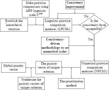
The framework of AHP with the PIS.
There are two differences between AHP with the PIS and the AHP with the fixed numerical scale (FNS): (1) consistency test. In the traditional AHP with a fixed numerical scale, the consistency test is conducted on NPCMs, and in the AHP with the PIS, it is to check the consistency of LPCMs; (2) the transformation process between LPCMs and NPCMs. In the AHP with the FNS, the transformation process is based on a certain numerical scale (e.g., the Saaty scale). In the AHP with the PIS, the transformation between LPCMs and NPCMs is conducted by the individual numerical scales.
(1) Consistency test regarding LPCMs
Up to now, a lot of works regarding the consistency issue of LPCMs have been reported (see [1], [44], [47] and [48]). In particular, transitive properties have been utilized to capture the consistency issues of LPCMs. Let L = (lij)n×n be as above. In the following, we introduce several transitive properties of L = (lij)n×n (see [18]):
a) Intransitivity. lij ≥ sg/2, ljt ≥ sg/2 ⇒ lit < sg/2 for ∀i, j, t.
Example 1.
Let L = (lij)3×3 be an LPCM over alternatives {x1, x2, x3}, and L is listed below.
In an LPCM L, x1 is moderately more important than x2, i.e., l12 = s10 > s8, and x2 is strongly plus more important than x3, i.e., l23 = s13 > s8, and x1 is moderately plus more important than x3, i.e.,l13 = s5 > s8. Thus, L is an LPCM with intransitivity.
b) Weak stochastic transitivity. lij ≥ sg/2, ljt ≥ sg/2, ⇒ lit ≥ sg/2 for ∀i, j, t.
Example 2.
Let L = (lij)3×3 be an LPCM over alternatives {x1, x2, x3}, and L is listed below.
In an LPCM L, x1 is moderately more important than x2, i.e., l12 = s10 > s8, x2 is strongly plus more important than x3, l23 = s13 > s8, and x1 is moderately plus more important than x3, l13 = s11 > s8. Thus, L is an LPCM with intransitivity. Weak stochastic transitivity.
c) Strong stochastic transitivity. lij ≥ sg/2, ljt ≥ sg/2 ⇒ lit ≥ max (lij, ljt) for ∀i, j, t.
Example 3.
Let L= (lij)3×3 be an LPCM over alternatives {x1, x2, x3}, and L is listed below.
In an LPCM L, x1, is moderately more important than x2, i.e., l12 = s10 > s8, x2, is strongly plus more important than x3, i.e., l23 = s13 > s8, and x1 is demonstrately more important than x3, i.e., l13 = s14 > max{s10, s13}. Thus, L is an LPCM with strong stochastic transitivity.
d) Additive transitivity.
Example 4.
Let L = (lij)3×3 be an LPCM over alternatives {x1, x2, x3}, and L is listed below.
In an LPCM L, x1 is moderately more important than x2, i.e., l12 = s10 > s8, x2 is strongly plus more important than x3, i.e., l23 = s13 > s8, and x1 very very strongly important than x3 i.e., l13 = s15 = Δ−1 (s10) + Δ−1(s13) – s8. Thus, L is an LPCM with additive transitivity.
Obviously, the condition of the additive transitivity is the most restrictive, and followed by the strong stochastic transitivity and the weak stochastic transitivity. Usually, if a set of pre-established transitive properties are satisfied, we then consider that the consistency level of an LPCM is acceptable. In this paper, we assume that the consistency level of an LPCM is acceptable when the weak stochastic transitivity is satisfied. To improve the consistency level of an LPCM, several approaches have been suggested (e.g., [4, 5, 47]).
(2) Consistency-driven approach to obtain the numerical scale with PIS
In the AHP, the LPCMs given by a decision maker are often transformed into NPCMs for implementing the computation operation. Clearly, both the LPCMs and NPCMs are the preferences associated with the same decision maker. Naturally, if the consistency level of LPCMs is acceptable, then the consistency level of the transformed NPCMs should be as better as possible. Following this idea, we put forward a consistency-driven approach to set numerical scale with PIS. In the consistency-driven approach, a two-stage based optimization model is established to generate the individual numerical scales. The first-stage optimization model is to minimize the overall inconsistency level of NPCMs that transformed from LPCMs, and the second-stage optimization model is to obtain the unique optimal solution by further optimizing the optimal solution(s) obtained from the first-stage model.
The consistency-driven approach is formally presented in Section 4.
Discussion. Clearly, the consistency-driven approach is a two-procedure based approach. In the work of Dong et al. [13], a two-procedure based approach is also reported to set numerical scales in the AHP. In the following, the differences between our proposal and the work of Dong et al. [13] are analyzed:
- (1)
The first procedure is the detection of the individual characteristics in Dong et al. [13], and the first procedure of our proposal is the consistency test of LPCMs.
- (2)
In the second procedure of Dong et al. [13], a nonlinear programming model is constructed to yield individual numerical scales by optimally matching the individual characteristics generated from the first procedure. In the second procedure of our proposal, a consistency-driven optimization model that minimizes the inconsistency index of the transformed NPCMs is built to produce the individual numerical scales. In addition, the consistency-driven optimization model is converted into a linear programming model that can be easily solved.
4. Consistency-driven methodology to deal with the PIS
This section presents a consistency-driven approach to address the PIS in AHP. Specifically, we propose a consistency-driven optimization model to yield the individual numerical scales in section 4.1. Moreover, we make some discussions regarding the optimal solution(s) derived from the consistency-driven optimization model.
4.1. Consistency-driven optimization model
Recall that
Before proposing the consistency-driven optimization model, the consistency index (CI) of a NPCM is introduced.
For a NPCM A = (aij)n×n, if ait ×atj = aij for ∀ i,j,t ∈ {1,2,…,n}, then A is a completely consistent NPCM. In this case, log(ait)+log(atj) = log(atj), ∀ i, j, t ∈ {1,2,…,n}. Further, we have
Definition 6:
The consistency level of NPCM A = (aij)n×n can be defined as follows:
Clearly, CL(A) ∈ [0,1]. The smaller the CL(A) value, the better the consistency level of A is.
Naturally, we hope that the transformed NPCMs
Meanwhile, the AHP numerical scale NSAHP should satisfy the following two conditions (described as (8) and (9)):
If we set
Take logarithms on both sides, (8)–(10) can be equivalently written as (11)–(13), respectively:
According to (7) and (11)–(13), we propose a consistency-driven optimization model:
In model (14), NSAHP (si) (i = 0,1,…, 16) are decision variables. Solving model (14) yields the AHP numerical scale NSAHP(si) (i = 0,1,…, 16). Based on the obtained NSAHP(si) (i = 0,1,…, 16), LPCMs can be transformed into NPCMs.
For convenience, let p(s) (s ∈ SAHP) be the position index of s. For instance, we have p(si) = i. Let Bi = log(NSAHP(si)), then model (14) can be written as the following model:
In the following, we propose a method to transform model (15) into a linear programming model, which is described as Theorem 1.
For simplicity, we set K = {1, …, m-1}, Nk = {1,...,nk} (k ∈ K), and
Theorem 1.
Let
Proof.
In model (16), constrains (16-1), (16-2), and (16-3) guarantee that
4.2. Further discussion
This section discusses the problem of uniqueness of optimal solution to model (14).
In Section 4.1, we can obtain the optimal solution(s) to model (14). Nevertheless, in some cases, the optimal solution(s) to model (14) may not be unique. In particular, some of them are unreasonable (in the sense of consistency). To demonstrate this issue, Example 5 is provided.
Example 5.
Suppose that there is a hierarchical structure (see Fig. 3), which consists of one goal {G}, three criteria {C1, C2, C3}, and three alternatives X = {x1, x2, x3}. The LPCMs given by a decision maker based on SAHP are listed as follows,
In this example, we set Δ = 0.4. Using model (14), we can obtain a set of optional solutions. Here, we only list two optimal solutions: Ω1: {NSAHP(1) (si), i = 0,1,…, 16} and Ω2: {NSAHP(2) (si), i = 0,1,…, 16}, and they are provided in Table 3.

The hierarchical structure in Example 5.
| 8 | 9 | 10 | 11 | 12 | 13 | 14 | 15 | 16 | |
|---|---|---|---|---|---|---|---|---|---|
| Ω1:NSAHP(si) | 1 | 2.29 | 2.29 | 3.57 | 4.38 | 5 | 7.28 | 7.28 | 9.19 |
| Ω2:NSAHP(si) | 1 | 2 | 2 | 3.60 | 4.51 | 5 | 7.03 | 7.03 | 9.6 |
The individual numerical scales in Ω1 and Ω2
Based on Ω1 and Ω2,
- (1)
the NPCMs
- (2)
the NPCMs
According to definition 6, we can obtain the consistency levels of the transformed NPCMs
|
|
|
|
|
|
|---|---|---|---|---|
| Ω1 | 0.08 | 0 | 0.05 | 0.14 |
| Ω2 | 0.06 | 0 | 0.09 | 0.12 |
The consistency levels of NPCMs under Ω1 and Ω2, respectively
Example 5 shows that: (1) the optimal solutions to model (14) are not unique; and (2)
Let M* be the optimal objective value to model (14), let Ω = {Ω1, Ω2,…,Ωn} (Ωr = {NSAHP(r)(s0), …, NSAHP(r)(s16)}, r = 1,2,…,n) be a set of optimal solutions to model (14) let
Further, model (17) can be rewritten as follows:
In model (18), NSAHP (si) (i = 0,…, 16) are decision variables. The constraints (18-1)–(18-5) guarantee that the optimal solutions of model (18) are subsets of the feasible solution of model (14), constraints (18-3), (18-4) guarantee that the AHP numerical scale NSAHP (si) (i = 0,…, 16) is ordered and reciprocal, constraint (18-5) is used to control the range of individual numerical scales.
Solving model (18) obtains the optimal individual numerical scales. Let p(s) (s ∈ SAHP) and Bi (i = 0,1, …,16) be as above. Model (18) can be equally written as model (19).
In model (19), Bi (i = 0,1,2,…,16) are the decision variables. Solving model (19) obtains the optimal solution Bi,* (i = 0,1,2,…,16) to Bi (i = 0,1,2,…,16). Further, we obtain the individual numerical scales by NSAHP (si) = eBi* (i = 0,1, 2,...,16).
Model (19) is a non-linear programming model. To solve model (19) easily, Theorem 2 is proposed to transform model (19) into a linear programming model.
Theorem 2.
Let
Proof.
Constraint (20-1) guarantees that
5. Practical example
In this section, a practical example that presented in Srdjevic [41] is used to show the application process of our proposal.
This example focuses on the issue of reservoir water allocated to multiple purposes. The hierarchical structure that described as Fig. 4 is used by a decision maker to select profitable purpose. The hierarchical structure is made up of three levels: the goal level, the criterion level and the alternative level. The LPCMs expressed by the decision maker are provided in Tables 5–10.

Reservoir storage allocation.
| Goal | National income | Regional gains | Balance of payment | Import substitution | Foreign exchange |
|---|---|---|---|---|---|
| National income | s8 | s9 | s12 | s10 | s9 |
| Foreign exchange | s7 | s8 | s14 | s10 | s10 |
| Balance of payment | s4 | s2 | s8 | s5 | s4 |
| Import substitution | s6 | s6 | s11 | s8 | s10 |
| Regional gains | s7 | s6 | s12 | s6 | s8 |
LPCM with respect to reservoir storage allocation
| National income | Electric power generation | Irrigation | Flood protection | Water supply | Tourism recreation | River traffic |
|---|---|---|---|---|---|---|
| Electric power generation | s8 | s12 | s10 | s13 | s14 | s12 |
| Irrigation | s4 | s8 | s2 | s7 | s9 | s9 |
| Flood protection | s6 | s14 | s8 | s14 | s10 | s11 |
| Water supply | s3 | s9 | s2 | s8 | s7 | s8 |
| Tourism recreation | s2 | s7 | s6 | s9 | s8 | s9 |
| River traffic | s4 | s7 | s5 | s8 | s7 | s8 |
LPCM with respect to national income
| Regional gains | Electric power generation | Irrigation | Flood protection | Water supply | Tourism recreation | River traffic |
|---|---|---|---|---|---|---|
| Electric power generation | s8 | s4 | s6 | s3 | s6 | s8 |
| Irrigation | s12 | s8 | s9 | s4 | s9 | s11 |
| Flood protection | s10 | s7 | s8 | s8 | s9 | s10 |
| Water supply | s13 | s12 | s8 | s8 | s8 | s14 |
| Tourism recreation | s10 | s7 | s7 | s8 | s8 | s12 |
| River traffic | s8 | s5 | s6 | s2 | s4 | s8 |
LPCM with respect to regional gains
| Balance of payment | Electric power generation | Irrigation | Flood protection | Water supply | Tourism recreation | River traffic |
|---|---|---|---|---|---|---|
| Electric power generation | s8 | s10 | s14 | s13 | s10 | s11 |
| Irrigation | s6 | s8 | s12 | s9 | s10 | s7 |
| Flood protection | s2 | s4 | s8 | s5 | s2 | s6 |
| Water supply | s3 | s7 | s11 | s8 | s7 | s9 |
| Tourism recreation | s6 | s6 | s14 | s9 | s8 | s9 |
| River traffic | s5 | s9 | s10 | s7 | s7 | s8 |
LPCM with respect to balance of payment
| Import substitution | Electric power generation | Irrigation | Flood protection | Water supply | Tourism recreation | River traffic |
|---|---|---|---|---|---|---|
| Electric power generation | s8 | s10 | s16 | s14 | s11 | s10 |
| Irrigation | s6 | s8 | s10 | s13 | s9 | s6 |
| Flood protection | s0 | s6 | s8 | s7 | s5 | s4 |
| Water supply | s2 | s3 | s9 | s8 | s3 | s3 |
| Tourism recreation | s5 | s7 | s11 | s13 | s8 | s7 |
| River traffic | s6 | s10 | s12 | s13 | s9 | s8 |
LPCM with respect to import substitution
| Foreign exchange | Electric power generation | Irrigation | Flood protection | Water supply | Tourism recreation | River traffic |
|---|---|---|---|---|---|---|
| Electric power generation | s8 | s11 | s13 | s14 | s9 | s9 |
| Irrigation | s5 | s8 | s9 | s9 | s8 | s6 |
| Flood protection | s3 | s7 | s8 | s9 | s3 | s8 |
| Water supply | s2 | s7 | s7 | s8 | s4 | s2 |
| Tourism recreation | s7 | s8 | s13 | s12 | s8 | s8 |
| River traffic | s7 | s10 | s8 | s14 | s8 | s8 |
LPCM with respect to foreign exchange
Firstly, we use model (14) to obtain the optimal objective value M *, and we further utilize model (20) to obtain the unique individual numerical scale of S AHP, which are listed in Table 11.
| si | s0 | s1 | s2 | s3 | s4 | s5 | s6 | s7 | s8 |
| NSAHP (si) | 0.11 | 0.12 | 0.15 | 0.18 | 0.22 | 0.27 | 0.38 | 0.62 | 1 |
| si | s9 | s10 | s11 | s12 | s13 | s14 | s15 | s16 | |
| NSAHP (si) | 1.6 | 2.6 | 3.66 | 4.66 | 5.6 | 6.6 | 8.01 | 9.4 | |
The individual numerical scales
Meanwhile, the LPCMs are transformed into NPCMs using the obtained numerical scales with the PIS. The transformed NPCMs are listed below:
From NPCMs
Subsequently, a global priority vector can be generated by synthesizing the local priority vectors using Eq. (4). The global priority vector of alternatives is listed below:
Then the ranking of alternatives can be derived from w : Electric power generation > Tourism recreation > River traffic > Flood protection > Irrigation > Water supply.
6. Simulation and comparison analysis
In this section, we present simulation and comparison analysis to discuss the validity of our proposal. Specifically, the comparison criteria are presented. Then, the simulation method is designed. Finally, the comparison results are analyzed.
6.1. Comparison criteria
The consistency is the basics of the preference relations, and we hope that the NPCMs transformed from the corresponding LPCMs are as consistent as possible. Thus, the consistency index of the transformed NPCM is an important criterion to evaluate the decision efficiency of the AHP model. The Saaty’s consistency index and geometric consistency index have been widely used in the AHP. Therefore, we use these two consistency indexes to measure the consistency level of transformed NPCM. Moreover, the deviation between a NPCM and its priority vector should be as smaller as possible. Thus, we define the deviation between a NPCM and its priority vector as a comparison criterion. The Euclidean distance and Manhattan distance have been widely used in decision making models, so we use these two distance measures to compute the deviation between a NPCM and its priority vector. Saaty’s consistency index has been introduced in Section 2. In the following, we present the geometric consistency index, Euclidean distance between a NPCM and its priority vector, and Manhattan distance between a NPCM and its priority vector.
(1) Geometric consistency index
Let A = (aij)n×n be a NPCM, and P = (p1,…, pn)T be the priority vector obtained from A. Crawford and Williams [9] proposed the geometric consistency index (GCI) for measuring the consistency level of the NPCM A = (aij)n×n:
Clearly, GCI(A) ≥ 0. GCI(A) = 0 indicates that the NPCM A is a completely consistent NPCM. The smaller GCI(A) value signifies the better consistency level of the NPCM A.
(2) Euclidean distance between a NPCM and its priority vector
The Euclidean distance [10], ED, between the NPCM A and its priority vector P is computed by:
Clearly, ED(A) ≥ 0. ED(A) = 0 indicates that the priority vector P is completely consistent with the NPCM A. The smaller ED(A) value indicates the better efficiency of the AHP model.
(3) Manhattan distance between a NPCM and its priority vector
The Manhattan distance, MD, between A and P is calculated by:
Clearly, MD(A) ≥ 0. MD(A) = 0 indicates that the priority vector P is completely consistent with the NPCM A. The smaller MD(A) value indicates the better efficiency of the AHP model.
6.2. Simulation method
In this section, we design simulation experiment to compare our proposal with the AHP with a fixed numerical scale (FNS) (i.e., the Saaty’s numerical scale). The basic idea of the simulation method is as follows:
We randomly and uniformly generate the LPCMs on a given hierarchical structure based on the linguistic term set SAHP = {s0, s1,…, s16}. Then, we take the generated LPCMs as the inputs of our proposal (i.e., the AHP with the PIS) and the AHP with the FNS, and we can obtain the average values of CR, GCI, ED, and MD for all NPCMs (i.e., ACR, AGCI, AED, and AMD) under these two approaches, respectively.
The simulation method is presented in Table 12.
| Input: m, nk (k = 1,…,m − 1),
|
| Output: ACR(PIS), AGCI(PIS), AED(PIS), AMD(PIS), ACR(FNS), AGCI(FNS), AED(FNS), AMD(FNS) values. |
| Step 1: Based on the established hierarchical structure, we generate
|
| Step 2: Taking the generated LPCMs
|
| Step 3: Using the fixed numerical scale,
|
| Step 4: Output ACR(PIS), AGCI(PIS), AED(PIS), AMD(PIS), ACR(FNS), AGCI(PIS), AED(FNS), and AMD(FNS). |
Simulation method
6.3. Comparison results
In this section, we set different parameter values for the simulation method to analyze the performance of our proposal.
We consider a hierarchical structure with three levels: goal level, criterion level and alternative level. In this case, m = 3 and n1 = 1. Let ∆ = 0.4, when setting different n2 and n3 values as the inputs of the simulation method, and we run it 1000 times to generate the average values of ACR, AGCI, AED, and AMD under our proposed approach (i.e., AHP with the PIS) and the existing AHP approach (i.e., AHP with the FNS), respectively, which are described in Figs. 5-8.
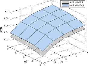
Average ACR value
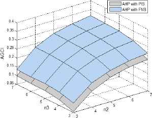
Average AGCI value
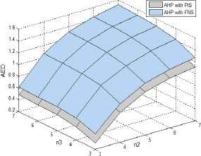
Average AED value

Average AMD value
From Figs. 5–8, we have the following observations.
The Saaty’s consistency index and geometric consistency index of the transformed NPCM, the Manhattan distance and Euclidean distance between a NPCM and its priority vector in the AHP with the PIS are obviously lower than those in the AHP with the FNS, respectively. This finding implies that the proposed approach can improve the decision efficiency by taking the PIS into account.
7. Conclusion
In the AHP, the PIS is an important factor that cannot be ignored due to its influence on the final decision results. This study proposes an AHP framework based PIS for supporting the decision making. The main work of this paper is summarized as follows:
- (1)
For implementing the computation process, in the AHP the linguistic preference information is often transformed into the numerical preference information using a fixed numerical scale function. In other words, the PIS is not considered by the existing AHP framework. By taking the PIS into account, this study proposes a novel AHP framework, which is closer to the realistic decision scenario.
- (2)
We develop a consistency-driven approach that minimizes the inconsistency level of the transformed numerical preference information (i.e., multiplicative preference relations) to support the proposed AHP framework. In the consistency -driven approach, a two-stage based optimization model is designed to deal with the PIS, and we transform it into linear programming model that can be easily solved.
- (3)
We design the detailed simulation experiment to verify the validity of the AHP framework with the PIS, and the simulation results show that our proposal has a better decision efficiency compared with the existing AHP framework.
Meanwhile, the following research paths are pointed out for the future:
- (1)
In our proposal, each element in an LPCM is mapped to an exact number. However, an LPCM is usually with uncertainty. To deal with this issue, the uncertain numerical scale (interval numerical scale) has been proposed and used in the linguistic decision making [19], further studies should discuss the uses of the interval numerical scale in the PIS based AHP framework.
- (2)
Practical decision making involves both mathematical models and psychological issues (e.g., prospect theory [17, 36]). However, psychological issues are seldom considered in the existing AHP models. To study the psychological issues of decision maker(s) in the PIS based AHP framework is a very interesting research direction.
- (3)
Acknowledgements
This work was supported by the grant (No. 71571124) from NSF of China, and the grant (No. 2017B07514) from “the Fundamental Research Funds for the Central Universities”.
References
Cite this article
TY  - JOUR
AU  - Qiuxiang Zhou
AU  - Yucheng Dong
AU  - Hengjie Zhang
AU  - Yuan Gao
PY  - 2018
DA  - 2018/01/01
TI  - The analytic hierarchy process with personalized individual semantics
JO  - International Journal of Computational Intelligence Systems
SP  - 451
EP  - 468
VL  - 11
IS  - 1
SN  - 1875-6883
UR  - https://doi.org/10.2991/ijcis.11.1.34
DO  - 10.2991/ijcis.11.1.34
ID  - Zhou2018
ER  -