
Personalized individual semantics based approach to MAGDM with the linguistic preference information on alternatives
- DOI
- 10.2991/ijcis.11.1.37How to use a DOI?
- Keywords
- Computing with words; multiple attribute group decision making (MAGDM); personalized individual semantics (PIS); numerical scale
- Abstract
Personalized individual semantics (PIS) exist widely in our daily life, and it means that different people have different understandings regarding the same word. In decision making, decision makers are accustomed to express their preferences using a linguistic way, and it is naturally that the PIS will influence the decision result in the linguistic decision making. In this paper, we propose a PIS-based MAGDM framework for multiple attribute group decision making (MAGDM) problems with the linguistic preference information on alternatives. In the novel framework, a two-stage based optimization model is constructed to deal with PIS by minimizing the deviation between objective preference information (i.e., multiple attribute decision matrix) and subjective preference information (i.e., linguistic preference relations over alternatives), and this optimization model is then transformed into a linear programming model that can be easily solved. Based on this, decision makers’ linguistic preference information can be transformed into numerical preference information for implementing the computation process. By fusing objective and subjective preference information, the collective solution of MAGDM problem can be obtained. The numerical and simulation experiments are conducted to verify the effectiveness of the proposal.
- Copyright
- © 2018, the Authors. Published by Atlantis Press.
- Open Access
- This is an open access article under the CC BY-NC license (http://creativecommons.org/licences/by-nc/4.0/).
1. Introduction
Multiple attribute decision making (MADM) refers to the problem of ranking alternatives from best to worst based on the multiple attribute decision matrix associated with multiple alternatives and attributes [7, 19]. The MADM has been widely used in many areas, such as economics, management, engineering and so on [4, 41]. As the decision-making environment becomes more and more complicated, it is hard for a single decision maker (DM) to take account all aspects of a decision making problem. In some situations, MADM problem needs to be solved by a group of DMs. Therefore, multiple attribute group decision making (MAGDM) models have been proposed and used to deal with the complex situations of decision making problems. In general, solving MAGDM problems includes the following two steps: (1) aggregating the individual multiple attribute decision matrices into a collective multiple attribute decision matrix; (2) obtaining the ranking of alternatives from collective multiple attribute decision matrix. The research on MAGDM has made a great progress, and the more information can be found in [11, 19, 42].
In the classical MAGDM problems, decision information only includes multiple attribute decision matrices that provided by a group of DMs. However, in some MAGDM problems, DMs will give preference information on alternatives besides multiple attribute decision matrices. This type of MAGDM problem is called MAGDM with preference information [20, 26]. Clearly, there are two kinds of preference information in MAGDM problem with preference information on alternatives: objective preference information (i.e., multiple attribute decision matrix) and subjective preference information (i.e., preference relations on alternatives). In the extant literature, Fan et al. [12] investigated MADM problem with fuzzy preference relation on alternatives. Moreover, Wang and Parkan [38] proposed some approaches to MADM with preference information, in which the attributes weights are incompletely known. Recently, Kadziński and Tervonen investigated MAGDM with additive value models and preference information on alternatives [20].
To our knowledge, most of the existing studies on MAGDM with preference information assumed that the DMs provide their preference information over alternatives using a numerical way [12, 26, 38]. However, in practice, some DMs may feel more comfortable to use a linguistic way to provide their preference information over alternatives instead of using a numerical way. In recent years, linguistic decision making has become a hot research topic in the decision area, and a lot of linguistic decision making models have been reported [5, 6, 9, 25, 31, 33, 34, 40, 47, 48]. When DMs use a linguistic way to provide preference information, it is natural that words mean different things for different DMs. In other words, DMs have personalized individual semantics (PIS) in linguistic decision making (e.g., [1, 27, 28]). PIS exist widely in our daily life. For example, during an interview, two interviewers both give comments “good” to an interviewee. However, the term “Good” may has different meanings, one interviewer may think this interviewee should score 80 points, while the other interviewer may think the interviewee should score 95 points, if using the hundred percentage point system. Therefore, PIS are important elements that cannot be ignored in linguistic decision making due to their influences on the final decision result. [21]. Recently, Li et al. [21] investigated the PIS in the group decision making with linguistic preference relations. The basic idea to deal with PIS presented in [21] is that if the consistency level of a linguistic preference relation is acceptable, then the consistency level of the numerical preference relation that converted from it should be as better as possible.
Surely, the PIS will also exist in MAGDM with linguistic preference information over alternatives. To our knowledge, there is no research that focused on this issue. To fill this gap, this paper proposes a PIS based framework for MAGDM problem with linguistic preference information on alternatives, which is inspired by the work of [21]. In the proposed framework, a two-stage based optimization model is proposed to yield the numerical scales of linguistic terms with PIS. In the first stage, an optimization model is designed to obtain the numerical scales of linguistic terms and the attributes weights by minimizing the deviation between objective (multiple attribute decision matrix) and subjective (linguistic preference relations over alternatives) preference information. However, the optimization model presented in first stage may have multiple solutions. To deal with this problem, the second-stage optimization model is presented to further optimize the solutions obtained from the first-stage optimization model. Both optimization models proposed in the first and second stages are transformed into linear programming models that can be easily solved. Based on this, the linguistic preference relations over alternatives are transformed into additive preference relations. Further, the collective solution can be obtained by fusing objective preference information (i.e., multiple attribute decision matrix) and subjective preference information (i.e., linguistic preference relations over alternatives).
Although the investigation of the PIS in our paper is inspired by the work of [21], the approaches to deal with PIS between them are clearly different. The approach to deal with PIS in [21] is based on consistency-driven methodology, while in our proposal, we address PIS by minimizing the deviation between objective preference information (i.e., multiple attribute decision matrix) and subjective preference information (i.e., linguistic preference relations over alternatives).
The rest of this paper is organized as follows. Section 2 introduces the 2-tuple linguistic model, numerical scale model and the MAGDM with numerical preference information on alternatives. In Section 3, a PIS based decision framework for MAGDM with linguistic preference on alternatives is proposed. The two-stage based optimization model is developed to support our framework, and a numerical example is used to show the applications of the proposed approach in Section 4. In Section 5, the numerical and simulation experiments are designed to verify the effectiveness of the proposal. Finally, concluding remarks are made in Section 6.
2. Preliminaries
This section provides some basic knowledge about the 2-tuple linguistic model, the numerical scale model, and the MAGDM problem with preference information on alternatives.
2.1 The 2-tuple linguistic model
This section introduces the 2-tuple linguistic model, which is the basis of numerical scale.
Zadeh [43] introduced the concept of linguistic variable as “a variable whose values are not numbers but words or sentences in a natural or artificial language”. A linguistic value is less precise than a number but it is closer to human cognitive processes used to solve successfully problems dealing with uncertainty. Let S = {si|i = 0, 1, 2,..., g} be a linguistic term set with odd cardinality. The term si represents a possible value for a linguistic variable, and it is required that the linguistic term set should satisfy the following characteristics [17, 43]:
- (1)
The set is ordered: si > sj if and only if i > j;
- (2)
There is a negation operator: Neg(si) = sj such that j = g − i.
The number of linguistic terms in the set S is called the cardinality of S. If the semantics of the elements in the linguistic term set are given by fuzzy numbers [36] (defined in the [0,1] interval), then the midterm represents an assessment of “approximately 0.5”.
Definition 1. [17]:
Let β ∈ [0, g] be a number in the Granularity interval of the linguistic term set S = {si|i = 0,1, 2,..., g}, and let i = round (β) and α = β − i be two values such that i ∈ [0, g] and α ∈ [−0.5, 0.5). Then, α is called a symbolic translation, with round being the usual rounding operation.
The 2-tuple linguistic representation model, presented in Herrera and Martínez [17] represents the linguistic information by a 2-tuple
Definition 2. [17, 24]
Let S = {si|i = 0, 1, 2,..., g} be a linguistic term set and β ∈ [0, g) be a value representing the result of a symbolic aggregation operation. The 2-tuple that expresses the equivalent information to β is then obtained as:
Function Δ, it is a one to one mapping whose inverse function
Definition 3. [8]
The matrix L = (lij)n×n, where lij ∈ S, is called a linguistic preference relation. The matrix L = (lij)n×n, where
In decision making with preference relation(s), the transitivity is an important concept. Let
- (1)
Intransitivity: lij > sα, ljk > sα ⇒ lki > sα for i, j, k ∈ {1,2,..., n}
- (2)
Weak stochastic transitivity: lij ≥ sα, ljk ≥ sα ⇒ lik ≥ sα for i, j, k ∈ {1,2,..., n}
- (3)
Strong stochastic transitivity: lij ≥ sα, ljk ≥ sα ⇒ lik ≥ max(lij, ljk) for i, j, k ∈ {1,2,...,n}
- (4)
Additive transitivity: lij = lik − ljk + sα for i, j, k ∈ {1,2,..., n}
Clearly, the additive transitivity condition is stronger than strong stochastic transitivity, and the strong stochastic transitivity condition is stronger than weak stochastic transitivity. In general, we consider that the linguistic preference relation is of acceptable consistency if it satisfies a set of pre-established transitive properties. In this study, we assume that the consistency level of the linguistic preference relation is acceptable if it satisfies the weak stochastic transitivity.
2.2 Numerical scale model
The concept of the numerical scale was introduced in [9], which is used to transform linguistic preference information into numerical preference for implementing calculation process.
Definition 4. [9]
Let S = {si|i = 0, 1, 2,..., g} be a linguistic term set, and R be the set of real numbers. The function: NS: S → R is defined as a numerical scale of S, and NS(si) is called the numerical index of si.
Definition 5. [9]
Let S,
2.3 MAGDM problem with numerical preference information on alternatives
The MAGDM problem with numerical preference information on alternatives is described as follows:
Let X = {x1, x2,..., xn} (n ≥ 2) be a finite set of alternatives, where xi denotes the i th alternative; E = {e1, e2,..., em} be a finite set of experts, where ek, (k = 1,2,..., m) denotes the k th expert; A = {a1,a2,...,at} (t ≥ 2) be a finite set of attributes, where aj denotes the j th attribute. Let V = (vij)n×t be a multiple attribute decision matrix, where vij is the preference value of the alternative xi with respect to the attribute aj. Let ω = (ω1, ω2,..., ωt)T be the attributes weight vector, where ωj ≥ 0 is the weight of attribute aj and
In extant literature regarding the MAGDM with preference information on alternatives, additive preference relations (also called fuzzy preference relations) are widely used. In addition, different preference relations can be transformed into other formats (see [14]). In the following, we introduce the additive preference relations in detail.
Definition 6. [15, 32]
A matrix P = (pij)n×n, where pij ∈ [0,1] and pij + pji = 1 for i.j = 1, 2,..., n, is called an additive preference relation over alternatives X = {x1, x2,..., xn}. Specifically, pij > 0.5 denotes that alternative xi is better than xj; pij < 0.5 signifies that alternative xj is better than xi; pij = 0.5 represents the equally importance between xi and xj.
Generally, ordinal and cardinal [3] consistency measures are two common types of consistency for a preference relation. The former is closely related to the transitivity of the corresponding preference relation, and the latter is a stronger concept because it not only implies the transitivity of preferences, but also the intensity of preference expressed by comparisons.
Similar to the transitive properties of linguistic preference relations, the transitive properties of additive preference relations are presented below:
- (1)
Intransitivity: pij > 0.5, pjk > 0.5 ⇒ pki > 0.5 for all i, j, k ∈ {1,2,..., n}
- (2)
Weak stochastic transitivity: pij ≥ 0.5, pjk ≥ 0.5 ⇒ pik ≥ 0.5 for all i, j, k ∈ {1,2,..., n}
- (3)
Strong stochastic transitivity: pij ≥ 0.5, pjk ≥ 0.5 ⇒ pik ≥ max(lij,ljk) for all i, j, k ∈ {1,2,..., n}
- (4)
Additive transitivity: pij = pik − pjk + 0.5 for all i, j, k ∈ {1,2,..., n}.
Based on additive transitivity, the cardinal consistency measure for an additive preference relation is presented below.
Definition 7. [16]
The cardinal consistency index (CCI) of an additive preference relation, P = (pij)n×n, is presented below:
3. A PIS based MAGDM framework
In this section, we propose a PIS based decision framework for MAGDM problem with linguistic preference information on alternatives.
3.1 The description of the problem: MAGDM with linguistic preference information on alternatives
As expounded in section 1, most of the studies assumed that the preference relations over alternatives in MAGDM were based on the numerical information. But sometimes in practical life, DMs may feel more comfortable to use a linguistic way to provide their preferences over alternatives. For implementing the calculation process, in linguistic decision making, the linguistic preference information is often transformed into the numerical preference information. When quantifying linguistic preference information, PIS are important elements that cannot be ignored due to their influences on the final decision. Based on above analysis, we present a new decision problem: MAGDM with linguistic preference information on alternatives, which is formally presented below.
Recall that E = {e1, e2,..., em} is a finite set of DMs; X = {x1, x2,...,xn} (n ≥ 2) is a finite set of alternatives; A = {a1, a2,...,at} (t ≥ 2) is a finite set of attributes; ω = (ω1, ω2,..., ωt)T is the weight vector over attributes A = {a1, a2,..., at}; and V = (vij)n×t is a decision matrix. Let λ = (λ1, λ2,..., λm)T be the weight vector of DMs, where λk ≥ 0 denotes the weight of DM ek and
In the decision making, DMs have PIS regarding their
3.2 The proposed framework
Here, we propose a new decision framework to handle MAGDM with linguistic preference relations on alternatives: PIS based MAGDM framework. This framework is described in Fig. 1, and two main steps are included in this framework: (1) transforming linguistic preference information into numerical preference information; (2) selection of the alternatives.
(1) Transforming linguistic preference information into numerical preference information
In this process, a consistency control process is utilized to improve the consensus level of linguistic preference relations. After that, a two-stage based optimization model is designed to yield the numerical scales with PIS by minimizing the deviation between objective (multiple attribute decision matrix) and subjective (transformed fuzzy preference relations over alternatives) preference information.
Note 1 : The numerical preference relations are widely used in GDM, such as multiplicative preference relations [3], additive preference relations [5, 16], and interval additive preference relations [5]. Herrera-Viedma et al. [14] discussed the transformation function between different numerical preference relations. The use of numerical preference relations will not change the essence of the proposed MAGDM framework. Without loss of generality, we consider that the linguistic preference relations are converted into additive preference relations in this paper.
The details of this process are presented in Section 4.
(2) Selection of the alternatives
After getting the numerical scales (NSk (si)) with PIS from the above step, we can transform the linguistic preference relations
Let OPV = (OPV1, OPV2,...,OPVn)T be the objective preference vector obtained from the multiple attribute decision matrix using Eq. (8), where OPVi represents the objective preference value from xi.
After getting the subjective and objective preference vectors, the collective preference vector, PV = (PV1, PV2,...,PVn)T, can be yielded, where the collective preference value of alternative xi is computed below:
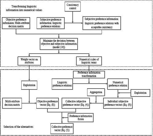
The PIS based MAGDM framework
Discussion. By taking the PIS into account, the deviation between objective and subjective preference information in our proposal can be decreased compared with the traditional MAGDM framework, which will be shown in the comparison section. Meanwhile, we should be noted that this paper assumes that linguistic preference relations provided by DMs are complete. However, in some situations, it may be difficult for DMs to provide all elements in linguistic preference relations on alternatives, which results in the uses of incomplete linguistic preference relations [35, 37, 39, 48]. In future research, we plan to investigate the management of incomplete linguistic preference relations under the PIS based MAGDM framework.
4. Obtaining the individual numerical scales with PIS
In this section, we propose a way to transform linguistic preference relations into numerical preference relations. Specifically, Section 4.1 proposes a basic model for obtaining the individual numerical scales with PIS. Section 4.2 further optimizes the basic model presented in Section 4.1. In addition, a numerical example is provided to illustrate our method in Section 4.3.
4.1 Modeling
Here, we propose a model to yield the individual numerical scales with PIS by minimizing the deviation between objective and subjective preference information. The model mainly includes three processes, which are presented below in detail.
(1) Obtaining objective preference vector from the multiple attribute decision matrix
In MAGDM problem, there are two categories of attributes: the benefit attributes and the cost attributes. Based on these two types of attributes, the multiple attribute decision matrix V = (vij)n×t is transformed into normalized multiple attribute decision matrix
Let OPV = (OPV1, OPV2,...,OPVn)T be as above, where the objective preference value of alternative xi is exploited by [19]:
(2) Obtaining subjective preference vectors from the preference relations over alternatives
Let
(3) Fusing the objective and subjective preference information
It is desirable that the deviation between the objective and subjective preference information is as small as possible. For DM ek, the deviation is calculated by
Further, Eq. (10) can be rewritten as follows:
Meanwhile, the numerical scales NSk (si), k = 1, 2,..., m should satisfy the following conditions:
(1) The numerical scale should be ordered, i.e.,
For controlling the discrimination degree between two consecutive numerical scales, we can take the following way:
(2) The numerical scale should be reciprocal, i.e.,
Moreover, for the flexibility of the numerical scales, we can set the range of NSk (si) as follows:
In this study, we consider that the attribute weights are unknown. Thus, the objective preference vector derived from Eq. (8) is also unknown. Based on the above analyses (Eqs. (10)–(15)), we establish an optimization model to calculate the individual numerical scales with PIS and attribute weights:
We denote this model as P1. By analyzing model P1, we present the following proposition.
Proposition 1.
Let NS(k, *) (si) be the optimal solution to decision variable NS(k)(si) in model P1. Let
Proof.
The Lk in model P1 satisfies the weak stochastic transitivity, from Definition 3, we have
Clearly, model P1 is a non-linear programming model. In the following, we transform it into a linear programming model that can be easily solved, which is shown in Theorem 1.
Theorem 1.
Let
Proof:
In the model (17), constrains (2)–(4) guarantee that
4.2 Further discussion regarding model P1
This section discusses the problem of uniqueness of solution to model P1
In Section 4.1, we obtain the optimal solution(s) to model P1. However, in some situations, the optimal solution(s) to P1 is not unique. Particular, some of the optimal solutions are not reasonable enough (in the sense of consistency). Here, we use an example, i.e., Example 1, to demonstrate this issue.
Example 1.
In this example, three DMs E = {e1, e2, e3}, four alternatives X = {x1, x2, x3, x4}, and three attributes A = {a1, a2, a3} are involved. The normalized multiple attribute decision matrix,
Miller [30] has demonstrated that an individual cannot simultaneously compare more than 7 ± 2 objects without confusion. The used linguistic term set with g+1 symmetry linguistic terms is a g / 2 +1 gradations. In this example the linguistic term set with 11 symmetry linguistic terms is used by DMs to express their preferences on alternatives.
S = {s0 = extremely poorer, s1 = much poorer, s2 = poorer, s3 = moderately poorer, s4 = weakly poorer, s5 = fair, s6 = weakly better, s7 = moderately better, s8 = better, s9 = much better, s10 = extremely better}
Meanwhile, the DM ek supplies the linguistic preference relation, Lk, based on linguistic term set S.
Here, we set γ = 0.05, Δ = 2,
| s0 | s1 | s2 | s3 | s4 | s5 | s6 | s7 | s8 | s9 | s10 | ||
|---|---|---|---|---|---|---|---|---|---|---|---|---|
| Ω1 | NS1(si) | 0.0783 | 0.1893 | 0.35 | 0.4 | 0.45 | 0.5 | 0.55 | 0.6 | 0.65 | 0.8107 | 0.9217 |
| NS2 (si) | 0.0754 | 0.1889 | 0.3492 | 0.3992 | 0.4492 | 0.5 | 0.5508 | 0.6008 | 0.6508 | 0.8111 | 0.9246 | |
| NS3 (si) | 0.0297 | 0.0939 | 0.2 | 0.25 | 0.3 | 0.5 | 0.7 | 0.75 | 0.8 | 0.9061 | 0.9703 | |
| Ω2 | NS1(si) | 0.2 | 0.2628 | 0.35 | 0.4 | 0.45 | 0.5 | 0.55 | 0.6 | 0.65 | 0.7372 | 0.8 |
| NS2(si) | 0.0788 | 0.2510 | 0.3492 | 0.3992 | 0.4492 | 0.5 | 0.5508 | 0.6008 | 0.6508 | 0.7490 | 0.9212 | |
| NS3(si) | 0.0310 | 0.0939 | 0.2 | 0.25 | 0.3 | 0.5 | 0,7 | 0.75 | 0.8 | 0.9061 | 0.9690 | |
The individual numerical scales in Ω1 and Ω2
Based on Ω1 and Ω2, we can transform L1, L 2 and L 3 into P 1, P 2 and P 3, respectively, and they are listed below:
(1) P1, P2 and P3 under Ω1
(2) P1, P2 and P3 under Ω2
According to definition 7, we can obtain the consistency levels of the transformed additive preference relations Pk (k = 1, 2, 3) under Ω1 and Ω2, respectively, which are listed in Table 2.
| P1 | P2 | P3 | |
|---|---|---|---|
| CCI(Pk under Ω1 | 0.1572 | 0.2755 | 0.2500 |
| CCI(Pk under Ω2 | 0.1167 | 0.2278 | 0.2500 |
The consistency levels of Pk (k=1, 2, 3) under Ω1 and Ω2, respectively
Example 1 shows that: (1) In some situations, optimal solutions to P1 are not unique; and (2) maxΩ1, k {CCI (Pk)} ≥ maxΩ2, k {CCI (Pk)}, this implies that the optimal solution Ω2 is better than Ω1 in the sense of consistency.
Therefore, it is necessary to further optimize the optimal solutions to P1. Let M* be the optimal objective function of model P1, and let Ω = {Ω1, Ω2,..., ΩT} be a set of optimal solution(s) to model P1. Then, using the optimization model,
Further, model (18) can be rewritten as follows:
In model (19), NSk (si) and ω = (ω1, ω2,..., ωt)T are decision variables. To solve model (19), Theorem 2 is presented.
Theorem 2.
By introducing a variable θ ≥ 0, then model (19) can be equally transformed into the following model:
Proof.
In model (20), constraint (1) guarantees that
Similar to the transformation process of model P1, model (20) can be transformed into a linear programming model that can be easily solved. For space limitations, we omit the transformation process of model (20).
4.3 Numerical example
In this section, we use a numerical example to verify the effectiveness of the proposed approach.
In this example, there are three DMs E = {e1, e2, e3}, four alternatives X = { x1, x2, x3, x4}, and four attributes A = {a1, a2, a3, a4}. In particular, a1, a3, a4 are benefit attributes, and a2 is a cost attribute. The multiple attribute matrix, V, is provided in Table 3.
| a1 | a2 | a3 | a4 | |
|---|---|---|---|---|
| x1 | 16 | 1 | 4 | 3 |
| x2 | 32 | 1 | 1 | 6 |
| x3 | 8 | 1 | 2 | 3 |
| x4 | 24 | 3 | 3 | 18 |
The multiple attribute decision matrix V
Meanwhile, DMs E = {e1, e2, e3} provide their linguistic preference relations {L1, L2, L3} on alternatives X = {x1, x2, x3, x4} using the following linguistic term set:
S = {s0 = extremely poorer, s1 = much poorer, s2 = poorer, s3 = moderately poorer, s4 = weakly poorer, s5 = fair, s6 = weakly better, s7 = moderately better, s8 = better, s9 = much better, s10 = extremely better}
The linguistic preference relations { L1, L2, L3} are listed below:
We set γ = 0.05, Δ = 2,
According to Eqs. (6) and (7), V is normalized into
The model P1 is used to get M* = 0.1792. Further, the individual numerical scales with PIS and attribute weights can be obtained by solving model (19), which are provided below:
Based on Table 4, the linguistic preference relations L1, L2 and L3 are transformed into additive preference relations P1, P2 and P3, respectively.
| s0 | s1 | s2 | s3 | s4 | s5 | s6 | s7 | s8 | s9 | s10 | |
|---|---|---|---|---|---|---|---|---|---|---|---|
| NS1(si) | 0.1 | 0.283 | 0.333 | 0.4 | 0.45 | 0.5 | 0.55 | 0.6 | 0.667 | 0.717 | 0.9 |
| NS2(si) | 0.2 | 0.25 | 0.35 | 0.4 | 0.45 | 0.5 | 0.55 | 0.6 | 0.65 | 0.75 | 0.8 |
| NS3(si) | 0.075 | 0.185 | 0.317 | 0.367 | 0.417 | 0.5 | 0.583 | 0.633 | 0.683 | 0.815 | 0.925 |
The individual numerical scales with PIS
Use Eq. (8) to yield the objective preference vector, OPV :
According to Eq. (9), we can obtain subjective preference vectors SPV(k) (k = 1,2,3) from additive preference relations Pk (k = 1,2,3), and they are listed below:
Following this, according to Eq. (4), the collective subjective preference vector SPV, can be obtained by aggregating SPV(1), SPV(2) and SPV(3) :
Further, the collective preference vector PV, can be obtained by fusing OPV and SPV using Eq. (5):
Based on PV, the ranking of the four alternatives can obtained, that is x1 > x4 > x2 > x3
5. Numerical and simulation analysis
In this section, we present several comparison criteria, and propose numerical and simulation analysis to discuss the validity of our proposal.
5.1 Comparison criteria
In the MAGDM with preference information on alternatives, there are two kinds of preference information, namely: objective and subjective preference information. Naturally, we hope that the objective and subjective preference information are as consistent as possible. Following this idea, we present the following criteria to evaluate the validity of our proposal: the deviation between the objective and subjective preference vectors, and the deviation between the objective and subjective preference rankings of alternatives [16, 45]. In the extant literature regarding the GDM, Manhattan distance and Euclidean distance have been widely used to measure the distance between preference vectors. Thus, Manhattan distance and Euclidean distance are adopted to measure the deviation between the objective and subjective preference vectors in this study. In addition, the consistency is a vital basis for GDM with preference relations. Thus, we consider the consistency of the transformed additive preference relations as a criterion to evaluate the validity of our proposal. The basic knowledge regarding the consistency issue of additive preference relations have been introduced in Definition 7 (section 2.3). The proposed comparison criteria except for the consistency of additive preference relations are introduced below.
(1) The Manhattan distance between the objective and subjective preference vectors
The Manhattan distance, MD, between the objective preference vector, OPV, and the subjective preference vector, SPV, is computed as follows:
(2) The Euclidean distance between the objective and subjective preference vectors
The Euclidean distance, ED, between the objective preference vector, OPV, and the subjective preference vector, SPV, is computed as follows:
(3) The deviation between objective and subjective preference rankings of alternatives
Let O = (o1, o2,..., on)T be the objective preference ordering derived from the objective preference vector OPV, where, if OPVi (i = 1, 2,..., n) is j largest in OPV, then oi = j (i = 1, 2,..., n). Using a similar way, the objective preference ordering
Let D [24] be the deviation between objective and subjective preference rankings of alternatives, which can be calculated by:
5.2 Numerical analysis
The existing approach for MAGDM with linguistic preference relations on alternatives is based on the fixed numerical scale. In our model P1, if the additive preference relation
The data used in this example is derived from Section 4.3. Using the fixed numerical scale, i.e.,
Taking
Based on the obtained attribute weights, the objective preference vector is obtained from Eq. (8),
According to Eq. (9), we can obtain subjective preference vector SPV(k) (k = 1, 2, 3) from additive preference relations
According to Eq. (4), the collective subjective preference vector SPV, can be obtained by aggregating SPV(1), SPV(2) and SPV(3).
Further, the collective preference vector PV, can be obtained by fusing OPV and SPV using Eq.(5):
Based on PV, the ranking of alternatives can be obtained, that is x4 > x1 > x2 > x3.
From this example and the numerical example presented in Section 4.3, we find that the collective solutions, i.e., the collective preference rankings of alternatives, under our proposal and traditional approach are different. This finding means that the PIS will influence the decision result. In the following, we compare these two approaches based on the four comparison criteria presented in Section 5.1. The comparison results are listed in Table 5.
| MD | ED | D | CCI | |
|---|---|---|---|---|
| MAGDM approach with PIS | 0.0472 | 0.0289 | 0 | 0.1148 |
| MAGDM approach with FNS | 0.1321 | 0.0802 | 0.5 | 0.1889 |
The comparison results between MAGDM approaches with PIS and FNS
From table 5, we find that our PIS based approach has a better decision efficiency under all criteria compared with the MAGDM approach with the fixed numerical scale.
5.3 Simulation analysis
(1) The comparison method
In this section, the existing approach for MAGDM with linguistic preference relations on alternatives is introduced. Then, a simulation method is designed to compare our proposal with the existing approach.
The basic idea of the simulation method is as follows:
We randomly generate the objective preference information V = (vij)n×t and subjective preference information
| Input: n, m, t, α λ = (λ1, λ2,..., λm)T and S = {sg | g = 0,1,..., g} |
| Output: D(PIS), D(FNS), ED(PIS), ED(FNS), MD(PIS), MD(FNS), CCI(PIS) and CCI(FNS). |
| Step 1: We generate multiple attribute decision matrix V = (vij)n×t and linguistic preference relations |
| Step 2: Use Eqs. (6) and (7) to transform V = (vij)n ×t into the normalized multiple attribute decision matrix |
| Step 3: Take |
| Step 4: Transform the linguistic preference information |
| Step 5: Output, D(PIS),D(FNS), ED(PIS), ED(FNS), MD(PIS), MD(FNS), CCI(PIS) and CCI(FNS). |
Simulation method
(2) Comparison results
Let S = {si | i = 0,1,2,...,10},
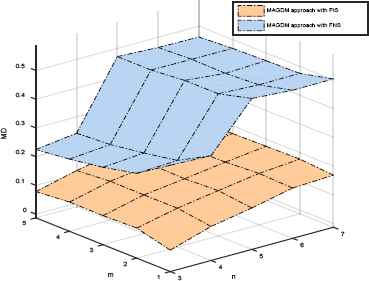
Average MD value
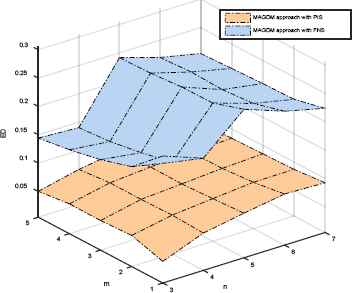
Average ED value

Average D value
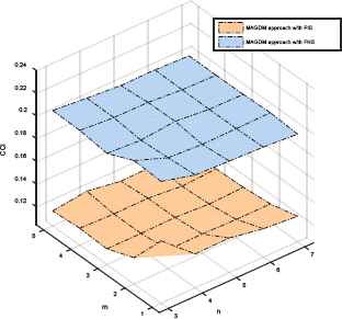
Average CCI value
From Figs. 2–5, we have the following observations. The Manhattan distance (MD) and Euclidean distance (ED) between the objective and subjective preference vectors, the deviation between objective and subjective preference rankings of alternatives (D), and the consistency of the transformed additive preference relations (CCI) in our proposed approach are obviously lower than those in the traditional approach with PNS, respectively. This finding implies that the proposed approach can improve the decision efficiency by taking PIS into account.
Note 2: In our proposal, the linguistic preference relations are transformed into additive preference relations, which are based on fuzzy numerical scales with PIS. So, we compare our proposal with the traditional method with fixed fuzzy numerical scales [12, 16, 17]. In the future, we plan to investigate the use of interval fuzzy numerical scales in the PIS based MAGDM framework, and compare it with the linguistic decision model with the fixed interval fuzzy numerical scales.
6. Conclusion
In this study, we propose a PIS based decision framework for MAGDM with linguistic preference relations on alternatives. The main points presented are as follows.
- (1)
The extant researches regarding the MAGDM with preference information on alternatives assumed that the DMs provide their preference information using a numerical way. This study assumes that DMs provide their preference information over alternatives using a linguistic way rather than a numerical way, which is closer to the realistic decision scenario.
- (2)
In decision making with linguistic preference information, PIS are important elements that cannot be ignored due to their influences on the final decision. This study takes the PIS into account, and proposes a PIS based MAGDM framework to improve the decision efficiency.
- (3)
We build a two-stage-based optimization model to obtain the unique individual numerical scale with the PIS. Moreover, we propose an approach to transform the proposed optimization-based optimization models into linear programming models that can be easily solved.
- (4)
We design detailed numerical and simulation experiments to verify the validity of the PIS based MAGDM framework. The numerical and simulation experiments show that our proposal has a better decision efficiency compared with the existing MAGDM framework.
Meanwhile, we argue that there are two interesting research paths for the future:
- (1)
In our proposal, each element in the preference relation is mapped to an exact number. However, the preference relation is usually with uncertainty. To deal with this issue, the uncertain numerical scale (interval numerical scale) has been proposed and used in the linguistic decision making [5], further studies should discuss the uses of the interval numerical scale in the PIS based MAGDM framework.
- (2)
Acknowledgements
This work was supported by the grant (No. 71571124) from NSF of China, and the grant (No. 2017B07514) from “the Fundamental Research Funds for the Central Universities”.
References
Cite this article
TY  - JOUR
AU  - Yuexuan Wang
AU  - Yucheng Dong
AU  - Hengjie Zhang
AU  - Yuan Gao
PY  - 2018
DA  - 2018/01/22
TI  - Personalized individual semantics based approach to MAGDM with the linguistic preference information on alternatives
JO  - International Journal of Computational Intelligence Systems
SP  - 496
EP  - 513
VL  - 11
IS  - 1
SN  - 1875-6883
UR  - https://doi.org/10.2991/ijcis.11.1.37
DO  - 10.2991/ijcis.11.1.37
ID  - Wang2018
ER  -