
A gene expression programming algorithm for discovering classification rules in the multi-objective space
- DOI
- 10.2991/ijcis.11.1.40How to use a DOI?
- Keywords
- Gene expression programming (GEP); Reference Point Based Multi-objective Evolutionary Algorithm (R-NSGA-II); Multi-objetive Evolutionary Algorithm (MOEA); Multi-objetive classification; Classification
- Abstract
Multi-objective evolutionary algorithms have been criticized when they are applied to classification rule mining, and, more specifically, in the optimization of more than two objectives due to their computational complexity. It is known that a multi-objective space is much richer to be explored than a single-objective space. In consequence, there are only few multi-objective algorithms for classification and their empirical assessed is quite limited. On the other hand, gene expression programming has emerged as an alternative to carry out the evolutionary process at genotypic level in a really efficient way. This paper introduces a new multi-objective algorithm for discovering classification rules, AR-NSGEP (Adaptive Reference point based Non-dominated Sorting with Gene Expression Programming). It is a multi-objective evolution of a previous single-objective algorithm. In AR-NSGEP, the multi-objective search was based on the well-known R-NSGA-II algorithm, replacing GA with GEP technology. Four objectives led the rules-discovery process, three of them (sensitivity, specificity and precision) were focused on promoting accuracy and the fourth (simpleness) on the interpretability of rules. AR-NSGEP was evaluated on several benchmark data sets and compared against six rule-based classifiers widely used. The AR-NSGEP, with four-objectives, achieved a significant improvement of the AUC metric with espect to most of the algorithms assessed, while the predictive accuracy and number of rules in the obtained models reached to acceptable results.
- Copyright
- © 2018, the Authors. Published by Atlantis Press.
- Open Access
- This is an open access article under the CC BY-NC license (http://creativecommons.org/licences/by-nc/4.0/).
1. Introduction
Classification is one of the most common tasks in machine learning and data mining. This task is required in many different application domains such as in medical diagnosis, patterns recognition, detection and prediction of failures in industrial applications, bank fraud prediction, text categorization, among others. This wide application spectrum is one of the reasons that has motivated for many years the development of new classifiers. In this sense, many and excellent algorithms have been proposed over the past years, examples include SVM1, ANNs2 and NB3. However, these proposals have the problem that the resulting learning model is like a black-box. On the other hand, there exists rule-based classifiers in the literature, e.g. CART4, ID35, CN26 and C4.57, which are more interpretable.
On the other side, mining rules with evolutionary algorithms allows interpretable classifiers to be designed; traditionally, they address the classification problem in a mono-objective manner, but the rule-based classifier can be tackled by means of using a multi-objective evolutionary algorithm (MOEA). It is a known fact that the accuracy and interpretability are conflicting objectives. Several works8,9 are asserting that it is unlikely to get good results in both kind of objectives. Then, a MOEA for the discovery of classification rules may find solutions with different trade-offs between these two kind of objectives. Some examples and state of the art in MOEAs are described in an extensive survey10. However, there are only few multi-objective algorithms for classification and their empirical assessment is quite limited11,12,13,14,15.
Evolutionary algorithms based their strength from two main sources: the exploration and the exploitation. But, as number of objectives grows, the classic Pareto dominance like NSGA-II16 and SPEA217 becomes ineffective to sort the quality of solutions since the population of non-dominated can be completely saturated. In this case, the genetic operators are innocuous to compensate that effect. Some studies have warned about this problem for several years18,19,20. On the other hand, in the real world optimization problems not all the objectives have the same importance and, therefore, the algorithms need to prioritize some of them over others and, additionally, during the evolutionary process may be necessary to change the priority of one or another objective18. To deal with these problems, in this work, we have taken into consideration the following capabilities in the AR-NSGEP and R-NSGEP (version with adaptability disabled) algorithms implementation:
- •
To avoid saturation of the population with non-dominated solutions.
- •
To find solutions with acceptable trade-offs between accuracy and interpretability.
- •
To change the level of importance among the objectives during evolutionary process (adaptive version).
- •
A new multi-objective algorithm for discovering classification rules by considering a GEP Michigan10 approach. The classifier is constructed as a decision list sorted by the rule-precision. The most numerous class in training was used as the default class. To avoid over-fitting, a threshold method was employed. Shortly, AR-NSGEP is a multi-objective evolution of the previous MCGEP21 algorithm.
- •
The mono-objective evaluation as well as the selection process of MCGEP were replaced by those considered in R-NSGA-II22 and NSGA-III23. A Token Competition was used to help the diversity control, maintaining a vector of the best non-redundant rules during every step of the evolutionary process. This strategy was used earlier in MCGEP with positive results.
- •
An adaptive algorithm so the importance of each objective is changed by considering the analysis of the best-rule movement in a ROC space. This procedure is carried out for each class and taking into account the kind of error that the best-rule movement causes.
- •
A GEP encoding following Ferreira24 definitions. We used a small but powerful arithmetic function set (+, *, −, /) to simplify the implementation of discriminant functions that encode the individuals in an expression tree form.
- •
An assessment carried out by scaling up to four the number of objectives for adaptive and non-adaptive versions of the multi-objective algorithm. Then, a comparative analysis is performed among the mono-objective MCGEP and the following versions: two objectives, three objectives and four objectives of AR-NSGEP and R-NSGEP.
- •
An assessment to verify the algorithm competitiveness versus other representative multi-objective algorithms (NSGA-II, SPEA2 and R-NSGA-II implemented as R-NSGEP). The experimental results on the real-world data sets showed the improvements of AR-NSGEP with respect to AUC and Accuracy metrics.
- •
An assessment to verify the algorithm competitiveness with other six Genetic Rule Based Systems (GRBS) algorithms referenced by the specialized literature. The experimental results achieved on different benchmark real-world data sets are also detailed in Section 6. After that, it is described how the proposed approach significantly improves the AUC and accuracy results in several cases. In this manner, the competitiveness of the proposed AR-NSGEP approach for mining classification rules is empirically demonstrated.
The remainder of the paper is organized as follows. In the next section 2, we review existing multi-objective evolutionary algorithms and previous applications related to the classification task; then, in Section 3, the components of the evolutionary algorithm are explained, several features such as the function set, the terminal set and the objectives calculation are also described in that section. In Section 4 the proposed multi-objective algorithm is presented, and the pseudo-code as well as the token competition for selecting the final solution obtained from the non-dominated front are described. The results are shown in Section 6; all experiments were performed on twenty-seven data sets. Finally, Section 7 offers some concluding remarks about the strength and weakness of the proposed algorithm as well as some future works.
2. Related work
This section focuses on the multi-objective evolutionary algorithms (MOEAs) and the formal Pareto definition. Then, different non-Pareto approaches are presented. Finally some MOEAs for classification problems are described.
2.1. Multi-objective evolutionary algorithms (MOEAs)
Most real-world decision problems require multi-objective optimization, which should be optimized simultaneously. Additionally, not any of the objectives have the same importance at any time18. Thus, the multi-objective optimization tries to find a set of solutions with an acceptable trade-off11,10, and there is not a clear criterion to compare all these solutions due to the relative importance among objectives is unknown or variable. Without loss of generality, a multi-objective optimization problem (MOP) can be stated as the maximization of the vector function:
Then, a concept of Pareto domination where a solution
- 1.
the solution
- 2.
the solution
The initial representative Pareto-based approaches of MOEAs (NPGA and NSGA) lack of elitism so they cannot guarantee that the non-dominated solutions obtained during the search process are always preserved. Later some elitist multi-objective algorithms were published, some of the most important are: SPEA2, PAES, and NSGA-II.
With the grow of objectives number, the classic Pareto dominance used in NSGA-II and SPEA becomes ineffective to sort the quality of solutions, in this case, the population of non-dominated can be completely saturated. Then, the genetic operators are unable to compensate that effect. To solve this problem many approaches make modifications of the classic Pareto dominance including some relaxed forms of Pareto such as ɛ-dominance and α-domination. The ɛ-dominance acts as an archiving strategy and was proposed as a way for regulating convergence. The α-domination permits a solution
2.2. Preference-based MOEA approaches
Another interesting way to address the multi-objective problem is to include preference information of an external decision maker. To the best of our knowledge, one of the first attempts to incorporate preferences in MOEAs was the work of Fonseca and Fleming27. Their proposal was an extension of MOGA to accommodate goal information as an additional criterion to non-dominance to assign ranks to the population. However, Thiele et al.19 proposed a preference-based evolutionary approach where at each iteration the decision maker is asked to give preference information in terms of a reference point. Cetkovic and Parmee28 converted fuzzy preferences into weights and a minimum threshold for dominance. Jin and Sendhoff 29 proposed a way to convert the fuzzy preferences in intervals of weights and using the method of dynamic weighted aggregation introduced in a previous work. This approach converts the multi-objective problem in a single-objective by aggregating the weights. In18 a new relationship of dominance called “superior strength” to replace classic Pareto dominance was proposed. It is based on information from the preference between objectives and it is constructed with a fuzzy inference system to find solutions in the preferable regions. González et al.9 work modified the crowding distance (CD) by Objective Scale Crowding Distance (OSCD). The parents selection technique was modified by a Crowding-Based Mating heuristic and the population size was dynamically adjusted. The Preference-based Interactive Evolutionary (PIE) algorithm20 used achievement scalarizing functions to help the decision maker to lead the search towards the desired Pareto optimal solution. Starting with approximation of the Nadir point. Guo and Wang30 proposed a new fuzzy multi-objective lattice order decision method for preference ranking in conflict analysis. In RP2-NSGA-II31 addressed the problem of multi-criteria ranking with a medium-sized set of alternatives as a multi-objective combinatorial optimization problem.
To develop this work we are inspired in Deb et al.22,23 and Yang et al.32 approaches. The R-NSGA-II and NSGA-III algorithms included preferences through reference points as well as a fast sorting scheme of non-dominated solutions and a modified crowding distance. The GrEA32 algorithm used the property of a grid to reflect the convergence and diversity information simultaneously. The performance of a solution regarding convergence can be estimated by the location of its grid compared to other solutions. The performance of a solution in connection to diversity can be estimated by the number of solutions with the same or similar grid location. In this work, Pareto-dominance was replaced by the Grid-dominance. This approach (x grid-domination) also balanced the diversity and convergence adaptively, varying the grid size.
2.3. MOEAs for classification
In a really interesting survey10, MOEAs for classification are categorized in three manners: evolving a good set of classification rules; defining the class boundaries (hyperplanes) in the training data; and modeling the construction of well known classifiers such as neural networks and decision trees. Our proposal is based on the first category by using a Michigan approach. Some major representative MOEAs for classification are described below.
In CEMOGA11, binary chromosomes of variable length are used to encode the parameters of a varied set of hyperplanes. It simultaneously minimizes the number of misclassified training points and the number of hyperplanes whereas the accuracy is maximized. In this work, authors proposed two quantitative scores: purity and minimal space for evaluating multi-objective techniques. A comparison was done with other classifiers in six UCI data sets: Vowel, Iris, Cancer, Landsat, Mango and Crude Oil.
EMOGA13 is a nonfuzzy categorical classification rule mining algorithm, proposed using an elitist multi-objective genetic algorithm and a weighted sum of three objectives. In this work the experimental section included Zoo, Nursery and Adult data sets obtained from UCI repository.
In the work propsoed by Satchidananda et al.12, an interesting multi-objective classification with gene expression programming was proposed. Here, two objectives were considered and the experimental section included two and three classes UCI data sets: Australian, Cloud, Cleveland, German data, Haberman, Heart, HouseVotes84, Iris, Pima and Wine. No comparison with other rule-based classifiers were done.
PAES-RCS14 generated a fuzzy rule-based classifier exploiting a multi-objective evolutionary algorithm. To learn the rule base they employed a rule and a condition selection approach. Two trade-offs objectives were used: accuracy and rule base complexity. The MOEA was tested by considering fifteen UCI data sets.
Cárdenas et al.15 proposed a multi-objective genetic process to generate fuzzy sets of rules. The algorithm was divided into three stages. The first one comprises the definition of an initial database with the same number of fuzzy sets for all attributes. The second and third stages were used for the rule generation and fuzzy sets optimization by means of multi-objective genetic algorithms to handle the accuracy-interpretability trade-off. The experimental section included seven UCI data sets: Iris, Wine, Thyroid, Heart, Sonar, Bupa and Breast.
3. Components of the evolutionary algorithm
Evolutionary algorithms (EAs) have been used over years to solve dissimilar classification problems in an accurate way. Two fundamental paradigms are highlighted: genetic algorithms (GAs) and genetic programming (GP). GP has been widely used in classification, several examples can be found in an extensive survey on the application of GP to classification33. Another emergent paradigm is gene expression programming (GEP)24 (GEP). In this paper we used GEP to encode individuals. In GEP, advantages of genetic algorithms (GA) and genetic programming (GP) are combined. The fundamental difference between these paradigms is located in the nature of individuals: in GA, symbolic fixed-length strings (chromosomes) were used; in GP, individuals are entities (trees) of varying size and shape; in GEP, individuals are also trees but they are encoded in a very simple way in the form of symbolic strings with fixed length. GEP includes a way to transform the string genes representation into trees such that any valid string generates a syntactically correct tree. In this paper the phenotype represents a discriminant function that is used to build a piece of the classifier. In GEP, genotype may be formed by several genes, each one divided into two parts: head and tail. The head of one gen will have a priori size chosen for each problem, and it contains terminal and non-terminal elements. The tail size, which may only contain non-terminal elements will be determined by the equation t = h * (n − 1) + 1, where t is the tail size, h is the head size and n is the maximum arity (number of arguments) in the non-terminal set. This expression ensures that, in the worst case, there will be sufficient terminals to complete the expression tree. Valid tree generation is a problem that may arise and should be treated in GP. Moreover, performing the evolutionary process at the genotypic level in a fixed-size string as in genetic algorithms (GAs) is more efficient than do it on a tree like in GP; these two are some of the fundamental advantages present in GEP.
3.1. Initial population
The generation of an initial population in GEP is a simple process. Here, it is only necessary to ensure that the head is generated with terminal and non-terminal elements and the tail only with terminal elements randomly taken from the element set (union of terminal and function set). The population size is defined in the popsize algorithm parameter.
3.2. Genetic operators
In GEP, there are several genetic operators available to guide the evolutionary process, which can be categorized into: mutation, crossover and transposition operators. Sometimes particular GEP transposition operators are included within the mutation category, and other specific GEP operators listed below are included within crossover category. In this work we used the following genetic operators: simple mutator (GEPSimpleMutt), transposition of insertion sequence (GEPISTranspositionMutator), root transposition of insertion sequence (GEPRISTranspositionMutator), one-point recombination (GEPOnePointRecombinator) and two-point recombination (GEPTwoPointsRecombinator). All of them were implemented as recommended by Ferreira24. A more detailed explanation of each one can be consulted in24 or in the previous MCGEP21 work.
3.3. Function set and terminal set
In this paper, we used the basic arithmetic operations to build the discriminant functions that form the final classifier as a decision list; the function set was formed by the following operations: * (multiplication), / (division), + (addition) and − (subtraction). In all the cases, these functions were established with arity = 2. By now, we implement an algorithm only for numerical data sets. Terminals are attributes or elements from constant list defined in the configuration file.
3.4. Fitness function
Each individual encodes a rule in Michigan-style, representing a discriminant function and having a class as the consequent. It represents, in each run of the algorithm, the current class, so the algorithm runs as many times as classes exist in an one-vs-all approach. In this multi-objective algorithm, we have several objectives included in the fitness function, the equations 5, 6, 7 and 8 were used for each one.
The first two objectives have also been widely used as performance metrics for rules. The third is a good metric for finding rules with which a decision list can be built. The last objective guarantees a good interpretability in the final model. The tp, tn, fn and fp represent: true positives, true negatives, false negatives and false positives respectively from the confusion matrix obtained from evaluating an individual in the training set, see the figure 1.
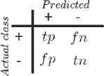
Confusion matrix.
The term phenotSize in equation 8, is the length (number of terminal and non-terminal elements) of the expression tree coded in the phenotype of an individual, this factor reaches its maximum unitary value when a phenotype is as simplest as possible (length equal to one). This factor was designed as a negative slope line decreasing to a minimum of 0.1 when the length reaches the maximum pheno-type represented by the value maxSize.
3.5. Classification with discriminant functions
Discriminant functions are one of the schemes used in data mining for rules classification. In a discriminant function, the output is computed as a value that is the result of evaluating the function on input attributes. Then, this value must be compared with a threshold (normally 0) to associate it with the corresponding initial pattern classification. A classifier will consist in a list of discriminant functions where each function associates an output class. For the two classes case, the classifier would be as in equation 9, where X is the input feature vector. In this case the function f (X) split the characteristic space only into two regions.
The multi-class problem can be solved by using one-vs-all approach (OVA) where the n-class problem is transformed into n two-class problems. In this approach the instances of each class is taken as positive instances and the rest as negative ones. On the other hand, a way to build the classifier would be: finding a single discriminant function for each class. However, it has the disadvantage that in real world problems the space of feature is usually much more complex. Thus we need to find more than one function for each class so the proposed algorithm searches for discriminant functions to achieve a certain predefined level of coverage over all the instances for each class. Thus, a decision list is generated where the best functions are placed first. When a new instance is presented to this classifier, the first function of the list is evaluated. If it returns a positive value, then the class associated with this discriminant function is returned. On the contrary, if it returns a non-positive value, then the next discriminant function is evaluated, and so on. If no one returns a positive value, the most numerous class in the training set is returned as default.
4. Proposed reference point based approach
This work is based on the innovative approaches R-NSGA-II22 and NSGA-III23. In our case, we are only interested in the search for nearby solutions to the ideal point for all objectives. In addition to a reference point multi-objective strategy, a token competition is carried out, where any objective of each individual is recomputed multiplying it by the rate between winning tokens and those that are possible to winning. A token is an instance of the training collection. Covered instances are removed from the competition. Redundant individuals obtain a low fitness (zero if they cover the same instances previously covered by others individuals in population), thus an individual with a good initial fitness (a set of all objectives) but with a low rate of new (not covered by others) won-tokens can leave the competition with low fitness and in the worst case with zero fitness. Before each competition, individuals are sorted according to their euclidean distance to the ideal objective point.
4.1. R-NSGEP algorithm
R-NSGEP is a first step that allows to reach the adaptive version named AR-NSGEP. As previously said, the R-NSGEP implementation is based on the MOEA (R-NSGA-II) approach of Deb et al.22 as starting point. Initially, parent and offspring populations are joined. Then a non-dominated sorting is performed to classify the combined populations into different levels of non-domination. Solutions from the best non-domination levels are chosen and a modified crowding distance operator is used to choose a subset of solutions from the last front until the population size is reached. The following steps are then performed:
- •
The normalized Euclidean distance is calculated from the ideal reference point to each front solution. With this, solutions are sorted in ascending order. The closest reference solution would be the first in crowding distance ranking. Solutions with a small crowding distance are preferred.
- •
To control the quantity of solutions obtained, all the solutions having a normalized euclidean distance between them and ɛ or less are grouped. A randomly picked solution from each group is retained and the rest of the members of the group are assigned with a large crowding distance in order to discourage them (see Figure 2). This ɛ strategy is similar to that suggested in34.
As shown in the pseudo-code (see Algorithm 1, line 4), the evolutionary process begins with the generation of the initial population bset with popsize. Then, an iterative process in the population starts for several generations until any of the following stop conditions are reached: the maximum number of generations gmax is perfromed, or an individual with fitness ≈ 1 is obtained. In each generation, individuals are evaluated according to the objective functions defined in the subsection 3.4 (see equations 5, 6, 7, 8). The selection procedure is detailed in the pseudo-code (see Algorithm 1, line 8).
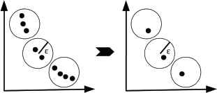
Epsilon reduction strategy.
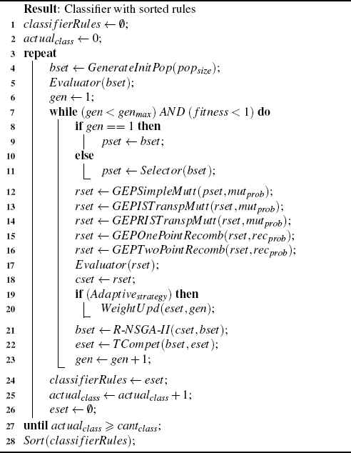
R-NSGEP, pseudo-code.
For each generation, we used the selection operator of the R-NSGA-II algorithm. This operator is based on a binary tournament, considering the fronts of non-dominance and the crowding distance. The crowding distance is also affected by the ɛ reduction strategy.
The GEP operators detailed in Section 3.2 are applied to the previously selected set of parents (pset), see lines 12 to 16; then, the obtained offspring (represented as rset) are evaluated as shown in line 16. Subsequently, on line 19, it is checked whether the adaptive strategy (AS) is performed. This AS is explained in the next section “AR-NSGEP. Adaptation with ROC analysis”. Parents and offspring are joined to be sorted in non-dominations fronts as R-NSGA-II does (see line 21). Then, a TCompet() (token competition) is performed on the union of the sets bset and eset. It returns a new non-redundant vector of individuals, eset as denoted line 21. The pseudo-code of this function is illustrated in Algorithm 2.
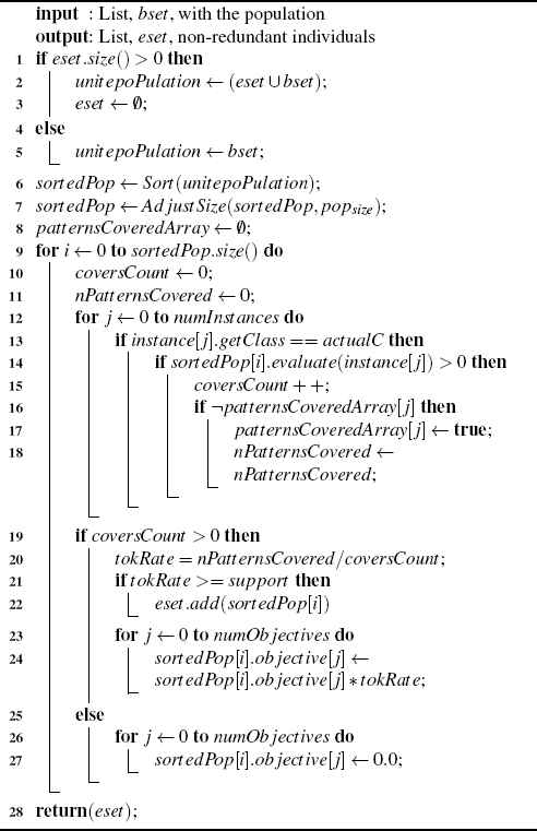
Function TCompet(bset).
After finishing a complete generation, the whole process (starting at line 7) is repeated until the maximum number of generations is reached or until an individual achieves a fitness very close to 1.0. Once any of the previous stop conditions is reached, all the elements within eset are added to the classifier and the algorithm is initialized with the next class, repeating the whole process (starting now from line 3 in the pseudocode). In each complete iteration of the algorithm the class used to calculate the fitness is assigned as consequent of the rule, assuming as positive instances those belonging to that class and as negative those belonging to the other classes. The algorithm is repeated as many times as number of classes exist in the training set, and each cycle adds to the classifier all the rules coded in eset individuals, which is reset to an empty list each time (see line 26). At the end of the process, all the rules in the classifier are sorted according to its value of precision on the training subset not covered by the previous precision-best rule (used initially the best precision-rule over full training set). Precision is computed as illustrated in equation 7.
5. AR-NSGEP. Adaptation with ROC analysis
Graphs of receiver operating characteristic (ROC) are widely used in the data mining field recently. ROC analysis has been used in the field of signal detection to describe the trade-off between true positive rate (TPR) and false positive rate (FPR)35. The work36 showed that only accuracy as a metric to measure the performance of a classifier is not always the best option. The ROC curves have the advantage of being a clear graphical representation and they are especially useful where exists in class distribution the imbalance problem35. After the explanation of the R-NSGEP algorithm in the previous section we can say that it is an application of the preference-based EMO approach (in particular R-NSGA-II) in the classification task, to use it in this context we made the following modifications:
- •
Token Competition to remove redundancy in the rule base that is used to build the classifier.
- •
Single ideal reference point (1; 1; 1; 1) to guide the search process.
- •
GEP technology for coding the individuals and genetic operators of this technology.
Wi (with value between 0.0 and 1.0) modifies the importance level of the Objectivei in the selection and fronts construction process. Wi can take the following shapes: Wsen for sensibility, Wspe for specificity, Wpre for precision and Wsim for simpleness. Another core issue of this new version was inspired in some ideas described in18 where it was stated that “during the evolutionary process may be necessary to change the priority of one or another objective”. To implement this idea, an adaptive strategy based on representation of a rule O in the ROC space (see Figure 3) is proposed.
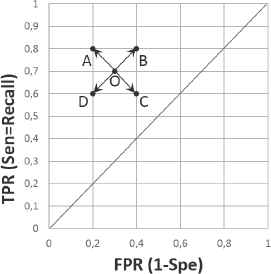
ROC analysis of the movement directions for the point O.
It is important to highlight that this process is performed for each class independently (we used OVA approach). During each evolutionary iteration, without loss of generality, we assume that an individual can move only in one of the four directions represented in Figure 3, where arrows would be the destination points A, B, C and D. In Figure 3, the Y axis as TPR = tp/(tp + fn) = Sensitivity and the X axis as FPR = fp/(fp +tn) = 1 − Specificity were plotted. Here, tp, fp, tn and fn are the counts in the confusion matrix shown in Figure 1.
We define ΔWi = Wi(g) − Wi(g − 1), where the current generation was represented by g and the previous generation with g − 1. i is the objective in consideration (sensibility, specificity, precision or simpleness), whereas tp + fn and fp +tn are constants. We can study four cases:
- •
When a rule moves from O to the point A in ROC space, we have a tp increment (+) and a fp decrement (−) at the same time. In this regard, we have a tn increment (+) and a fn decrement (−). It means that the rule evolved in a very good direction. Then, AR-NSGEP slows down the exploration (lesser steps), to focus in that vicinity. This is achieved by making ΔWspe, ΔWpre and ΔWsen lower than zero and, then, substituting the new Wi value for each objective in the equation 10.
- •
When a rule moves from O to the C point, we have a tp decrement (−) and a fp increment (+) at the same time. As a consequence, there is a tn decrement (−) and a fn increment (+). In this case, the rule evolution is very bad in both directions. Then, AR-NSGEP takes the decision of an exploration increment to get away of that vicinity. This is achieved by making ΔWspe, ΔWpre and ΔWsen greater than zero.
- •
When a rule moves from O to the B point, then we have a tp increment (+) and a fp increment (+) at the same time. As a consequence, we have a tn decrement (−) and a fn decrement (−). In this case, the rule evolution is good in Sensibility = TPR direction but bad in Specificity = 1 − FPR direction. Then, AR-NSGEP slows down the searching for objective sensibility and speeds up exploration for specificity. This is achieved making ΔWspe and ΔWpre greater than zero and ΔWsen lower than zero.
- •
Finally, when a rule moves from O to the D point, we have the opposite of the previous case. AR-NSGEP speeds up exploration for sensibility objective and slows down the exploration for specificity objective. This is achieved by making ΔWspe and ΔWpre lower than zero and the ΔWsen greater than zero.
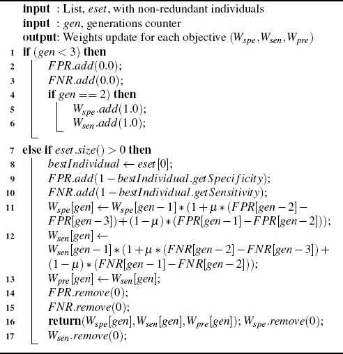
Function WeightU pd(eset, gen)
We can note that a good metric to automatically adapt the parameters ΔWspe and ΔWsen can be the following: ΔFPR = FPR(g) − FPR(g − 1) and ΔFNR = FNR(g) − FNR(g − 1), respectively. For ΔWpre we also used ΔFPR. This new WED (see equation 10) guides the searching process during the evolutionary process as the R-NSGEP algorithm explained in the previous Section 4. Finally, we introduced a momentum factor in AR-NSGEP. The gradient algorithm with momentum has been widely used for neural networks training for many years2. The momentum coefficient is selected as a positive constant in the interval (0, 1). It is considered a technique that may help out from local minims. The momentum has the effect of damping oscillations in the training of weights. Momentum simply adds a fraction μ of the previous weight update to the current one. When the weight update keeps pointing in the same direction, this will increase the size of the steps taken towards the minimum. Therefore, we have introduced this factor in the weights updating process as shown in equations 11, 12 and 13. These equations and this adaptive strategy were implemented with the function WeightU pd() invoked in line 20 of Algorithm 1, see pseudo-code in Algorithm 3.
Note that, during the first three generations, weights are not updated. Tu sum up, in the AR-NSGEP adaptive version we use the NSGA-III reference point approach, taking the ideal point for all objectives. However, to follow the best individual of the population in its movement for the ROC space, we modify the Wi importance level for each objective. At the same time, the searching process is adjusted to make it more intense when there exist movement in a good direction and more extensive in the opposite case.
6. Empirical evaluation
This section presents the experimental methodology followed to assess the proposed AR-NSGEP algorithm. Three different experiments were performed. In the first experiment, we compared seven GEP-based algorithms. A single-objective (MCGEP) algorithm and another six versions with two, three and four objectives of the R-NSGEP and AR-NSGEP approaches. Each one was named as follows: two-objective versions (R-NSGEP-2 and AR-NSGEP-2); three-objective (R-NSGEP-3 and AR-NSGEP-3); and the four-objective versions (simply named as R-NSGEP and AR-NSGEP).
As the evolutionary process is dependent on the MOEA it includes, then the second experiment is responsible for evaluating the performance of our previous best proposals against three well known MOEAs. In the last experiment, we evaluated the performance of our best proposal against six widely-known GP techniques for discovering classification rules that represent a large variety of learning paradigms. The methods used in the last comparison were: UCS, GASSIST, HIDER, SLAVE, LOGIT-BOOST, CORE. A more detailed explanation of each of the first six algorithms above can be found condensed in an excellent review37. The following subsection provides details of the real-world problems chosen for the experiments, the experimental tools and configuration parameters as well as the results and statistical tests applied to compare them.
6.1. Training sets
To evaluate the behavior of our classifier, twenty-seven real-world data sets were chosen from KEEL*38 and UCI†39 repositories. To execute the experiments, data sets listed in Table 1 were used.
| Id. | Data set | Inst. | Attrib. | Class |
|---|---|---|---|---|
| app | Appendicitis | 106 | 9 | 2 |
| aus | Australian | 690 | 14→18 | 2 |
| aut | Automobile | 159 | 25 | 6 |
| bal | Balance | 625 | 4 | 3 |
| ban | Banana | 5300 | 2 | 2 |
| bad | Bands | 365 | 19 | 2 |
| bup | Bupa | 345 | 6 | 2 |
| cle | Cleveland | 297 | 13 | 5 |
| con | Contraceptive | 1473 | 9 | 3 |
| der | Dermatology | 358 | 34 | 6 |
| eco | Ecoli | 336 | 7 | 8 |
| gla | Glass | 214 | 9 | 7 |
| hab | Haberman | 306 | 3 | 2 |
| hea | Heart-s | 270 | 13 | 2 |
| hep | Hepatitis | 80 | 19 | 2 |
| ion | Ionosphere | 351 | 33 | 2 |
| iri | Iris | 150 | 4 | 3 |
| lym | Lymphography | 148 | 18→38 | 4 |
| pim | Pima | 768 | 8 | 2 |
| son | Sonar | 208 | 60 | 2 |
| thy | Thyroid | 7200 | 21 | 3 |
| wdb | Wdbc | 569 | 30 | 2 |
| win | Wine | 178 | 13 | 3 |
| wis | Wisconsin | 683 | 9 | 2 |
| wpb | Wpbc | 194 | 32 | 2 |
| yea | Yeast | 1484 | 8 | 10 |
| zoo | Zoo | 101 | 17→21 | 7 |
Data set characteristics.
In our experimental assessment, all the examples with missing values were removed from the datasets. In Australian, Lymphography and Zoo datasets nominal attributes were binarized. In total, we have 14 binary problems, 5 three-class problems and 8 problems including between 5 and 10 classes. The evaluation of the quality of a classification algorithm may be seen as a multi-objective problem40 so we used three metrics for the assessment. We evaluated the performance of models evolved by each learning system with the test accuracy metric (proportion of correct classifications over previously unseen examples), AUC (area under ROC curve) and number of rules of the models obtained in each case. We used a ten-fold cross validation procedure with 5 different random seeds over each data set.
6.2. Experimental tools
We used the JCLEC‡ framework described in41, a software system for Evolutionary Computation (EC) research, developed in Java programming language. The parameters used in the algorithm are summarized in Table 2.
| Parameter | Value |
|---|---|
| Population size (popsize) | 500 |
| Maximum of generations (genmax) | 100 |
| Threshold support (support) | 0.01 |
| GEPSimpleMutator (mutprob) | 0.10 |
| GEPISTranspositionMutator (mutprob) | 0.10 |
| GEPRISTranspositionMutator (mutprob) | 0.10 |
| GEPOnePointRecombinator (recprob) | 0.40 |
| GEPTwoPointsRecombinator (recprob) | 0.40 |
| Epsilon non-domination reduction factor. (ɛ) | 0.01 |
| Mu. Damping factor. (μ) | 0.9 |
AR-NSGEP sumary parameters.
In our experiments, we used the chromosome size and constants list problem-dependent. The list of constants was fixed for all data sets except for the case of bands, pima and wine. In these cases, the constant values were different due to those data sets have attributes in a wide range of values. Note that no additional parameter optimization was done for R-NSGEP and AR-NSGEP. Thus, the configuration used for this algorithm should not be taken as the optimal set of parameters for each data set. Considering a particular dataset, a fine tuning may achieve even better results. The configuration files for AR-NSGEP and complementary material of the experimental study are publicly available at the link.§
The way in which the size of the head in GEP is defined is still an open issue24, so we have adjusted this parameter through trial and error with values equal to ten times the number of attributes for each dataset. The source codes and optimum configurations for CORE, GASSIST, HIDER, SLAVE, UCS and LOGIT-BOOST were based on KEEL38 and their original authors as well as in the useful review37.
6.3. Statistical analysis
We followed the recommendations pointed out by Derrac et al.42 to perform the statistical analysis of the results. As the authors suggested, non-parametric statistical tests are used to compare the accuracy and sizes of the models built by the different learning systems. Specifically, we used Friedman’s test. Derrac et al.42 found in their work that Finner and Li tests denoted the most powerful behavior, reaching the lowest p-values in the comparisons. Then, we applied these tests to arrive at solid conclusions. To statistical computations we used the “scmamp” library43 implemented with the R programming language.
6.4. Experiment #1
In this experiment we analyze the behavior of the proposed algorithm for two, three and four objectives. The previous mono-objective version, MCGEP, is also included in this comparison. The average results for each collection are shown in Table 3. The last row shows the average rank for each algorithm.
| Data Sets | MCGEP | R-NSGEP-2 | AR-NSGEP-2 | R-NSGEP-3 | AR-NSGEP-3 | R-NSGEP | AR-NSGEP | ||||||||||||||
|---|---|---|---|---|---|---|---|---|---|---|---|---|---|---|---|---|---|---|---|---|---|
| Acc | AUC | NR | Acc | AUC | NR | Acc | AUC | NR | Acc | AUC | NR | Acc | AUC | NR | Acc | AUC | NR | Acc | AUC | NR | |
| app | 83.60 | 74.56 | 6.92 | 81.89 | 62.94 | 33.80 | 81.84 | 63.07 | 33.84 | 83.42 | 74.54 | 7.62 | 83.07 | 73.01 | 7.56 | 85.38 | 75.38 | 8.36 | 85.33 | 75.74 | 8.34 |
| aus | 84.84 | 85.00 | 8.94 | 81.54 | 81.03 | 146.72 | 82.43 | 81.92 | 147.46 | 85.39 | 85.47 | 9.72 | 86.52 | 86.43 | 10.10 | 85.48 | 85.46 | 11.26 | 85.54 | 85.64 | 11.62 |
| aut | 53.23 | 88.79 | 17.82 | 63.68 | 91.69 | 66.28 | 65.74 | 91.78 | 66.70 | 48.28 | 86.33 | 14.88 | 49.92 | 87.47 | 14.48 | 56.76 | 89.26 | 20.12 | 56.49 | 88.93 | 19.98 |
| bal | 96.51 | 95.96 | 7.12 | 89.85 | 85.31 | 81.56 | 90.12 | 85.19 | 80.22 | 89.72 | 82.46 | 8.00 | 88.86 | 81.20 | 8.10 | 94.05 | 90.11 | 8.54 | 92.95 | 87.87 | 8.84 |
| ban | 82.62 | 82.02 | 9.18 | 87.55 | 87.18 | 114.08 | 87.56 | 87.20 | 114.24 | 76.54 | 75.59 | 9.24 | 77.13 | 76.32 | 9.20 | 81.97 | 81.35 | 10.76 | 82.15 | 81.64 | 10.90 |
| bad | 61.75 | 57.08 | 10.00 | 61.90 | 60.18 | 153.12 | 62.27 | 60.23 | 150.48 | 62.90 | 58.76 | 10.84 | 61.70 | 57.26 | 10.58 | 63.63 | 59.97 | 12.30 | 63.64 | 59.32 | 12.32 |
| bup | 68.78 | 67.22 | 10.42 | 63.01 | 62.21 | 123.12 | 61.70 | 60.99 | 123.64 | 65.22 | 63.34 | 10.28 | 65.96 | 64.10 | 10.68 | 67.48 | 66.00 | 13.56 | 67.93 | 66.33 | 13.44 |
| cle | 55.32 | 72.50 | 16.46 | 52.33 | 69.62 | 146.18 | 53.40 | 67.91 | 145.36 | 56.04 | 71.07 | 16.08 | 55.38 | 70.49 | 16.44 | 56.09 | 70.40 | 20.50 | 57.16 | 71.11 | 20.24 |
| con | 51.16 | 65.78 | 20.34 | 46.11 | 60.96 | 318.92 | 47.19 | 62.38 | 314.24 | 50.18 | 64.21 | 19.12 | 50.48 | 64.36 | 19.52 | 51.36 | 66.25 | 24.82 | 51.68 | 66.56 | 25.02 |
| der | 94.69 | 98.70 | 10.34 | 92.22 | 97.59 | 40.98 | 92.15 | 97.42 | 39.28 | 93.60 | 98.36 | 10.38 | 93.00 | 98.23 | 10.48 | 94.39 | 98.66 | 12.56 | 95.41 | 98.84 | 12.60 |
| eco | 69.76 | 93.27 | 17.14 | 59.83 | 92.45 | 148.28 | 58.69 | 92.14 | 150.60 | 65.60 | 92.64 | 17.30 | 66.39 | 92.25 | 17.32 | 73.41 | 94.81 | 22.66 | 71.10 | 94.30 | 22.14 |
| gla | 64.49 | 90.14 | 14.94 | 57.68 | 88.06 | 93.18 | 58.63 | 88.74 | 93.16 | 62.90 | 89.39 | 14.70 | 62.27 | 89.74 | 14.96 | 63.59 | 89.69 | 19.94 | 64.60 | 90.12 | 19.56 |
| hab | 72.02 | 63.26 | 8.92 | 72.55 | 59.84 | 62.20 | 71.76 | 59.23 | 61.72 | 72.11 | 63.12 | 9.56 | 73.55 | 64.63 | 9.32 | 72.76 | 64.52 | 10.50 | 72.11 | 63.93 | 10.30 |
| hea | 79.63 | 79.03 | 8.40 | 73.26 | 72.00 | 100.64 | 72.37 | 71.02 | 99.64 | 79.93 | 79.35 | 9.72 | 79.04 | 78.25 | 9.54 | 80.81 | 80.23 | 11.32 | 80.37 | 79.97 | 11.50 |
| hep | 86.00 | 76.25 | 5.80 | 75.64 | 72.43 | 18.52 | 76.77 | 73.50 | 18.28 | 86.97 | 78.49 | 5.84 | 88.11 | 78.54 | 5.74 | 84.80 | 74.14 | 6.38 | 87.23 | 77.15 | 6.26 |
| ion | 86.62 | 83.11 | 6.06 | 87.13 | 84.87 | 64.38 | 87.87 | 85.09 | 66.82 | 86.10 | 82.88 | 8.74 | 86.21 | 83.07 | 8.96 | 86.79 | 84.04 | 10.46 | 87.35 | 84.85 | 10.84 |
| iri | 95.87 | 97.93 | 4.84 | 96.00 | 98.00 | 13.16 | 96.40 | 98.20 | 13.20 | 92.93 | 96.47 | 4.58 | 95.33 | 97.63 | 4.88 | 95.47 | 97.67 | 5.38 | 96.53 | 98.23 | 5.30 |
| lym | 78.80 | 93.83 | 17.24 | 70.49 | 90.57 | 53.36 | 70.34 | 90.81 | 52.88 | 81.38 | 95.23 | 10.54 | 80.96 | 95.35 | 10.46 | 79.77 | 94.32 | 12.10 | 81.01 | 95.18 | 12.04 |
| pim | 66.21 | 62.04 | 11.44 | 69.87 | 65.85 | 165.76 | 68.54 | 64.38 | 160.08 | 72.76 | 70.07 | 11.72 | 71.91 | 68.72 | 11.32 | 72.17 | 68.99 | 13.60 | 73.37 | 70.01 | 13.78 |
| son | 67.93 | 67.47 | 9.72 | 61.90 | 62.93 | 106.38 | 63.90 | 64.84 | 103.64 | 71.84 | 71.40 | 9.30 | 71.13 | 70.75 | 9.46 | 68.86 | 68.43 | 10.50 | 69.54 | 69.04 | 10.56 |
| thy | 94.81 | 79.28 | 7.44 | 95.92 | 86.85 | 165.04 | 95.81 | 87.12 | 166.62 | 94.26 | 76.69 | 9.72 | 94.15 | 73.86 | 9.54 | 95.91 | 88.02 | 12.00 | 95.78 | 87.93 | 12.14 |
| wdb | 93.74 | 92.92 | 6.06 | 90.64 | 91.00 | 98.34 | 89.84 | 90.46 | 98.40 | 93.04 | 92.13 | 6.10 | 93.11 | 92.30 | 6.16 | 93.42 | 92.74 | 7.18 | 93.88 | 93.13 | 7.08 |
| win | 90.88 | 95.73 | 6.76 | 82.99 | 91.00 | 36.04 | 84.92 | 92.16 | 35.24 | 87.71 | 93.94 | 7.98 | 89.17 | 94.57 | 7.86 | 92.14 | 96.07 | 7.86 | 94.60 | 97.40 | 8.08 |
| wis | 95.59 | 95.65 | 3.92 | 93.48 | 92.17 | 80.08 | 93.22 | 91.80 | 77.18 | 94.54 | 94.10 | 5.10 | 94.06 | 93.54 | 5.02 | 95.56 | 95.27 | 5.10 | 95.62 | 95.32 | 5.40 |
| wpb | 70.13 | 57.30 | 10.06 | 62.08 | 53.06 | 93.30 | 62.97 | 54.11 | 93.60 | 70.42 | 54.80 | 11.28 | 70.68 | 56.53 | 10.98 | 70.61 | 56.63 | 11.00 | 72.06 | 57.77 | 11.38 |
| yea | 49.58 | 86.76 | 36.04 | 45.85 | 87.10 | 513.42 | 46.40 | 87.35 | 505.44 | 48.10 | 85.73 | 36.90 | 48.24 | 85.62 | 37.56 | 54.53 | 89.58 | 53.80 | 54.42 | 89.71 | 55.14 |
| zoo | 94.60 | 98.71 | 7.34 | 91.44 | 98.04 | 9.98 | 91.62 | 98.04 | 10.12 | 93.49 | 98.43 | 7.26 | 92.33 | 98.14 | 7.26 | 94.24 | 98.62 | 8.66 | 95.24 | 98.88 | 8.78 |
| Rank | 3.74 | 3.44 | 1.70 | 5.44 | 5.35 | 6.56 | 5.37 | 5.17 | 6.44 | 4.39 | 4.48 | 2.26 | 4.33 | 4.41 | 2.22 | 2.78 | 3.04 | 4.26 | 1.94 | 2.11 | 4.56 |
Accuracy (Acc), area under ROC curve (AUC) and rule set length (NR) comparative results.
The multi-comparison Friedman’s test rejected the following null hypotheses: all the systems performed the same on accuracy (Acc) with Friedman’s p – value = 1.1826 × 10⁻¹⁰; all the systems performed the same on AUC with Friedman’s p – value = 9.2003 × 10⁻⁹ and the number of rules in the models was equivalent on average with Friedman’s p – value = 7.3714 × 10⁻¹¹. To check the results, we apply Finner’s and Li’s methods to test the hypotheses ordered by their significance. As can be seen in Table 4, all tests with α = 0.05 detect a significant difference in Acc performance of AR-NSGEP against the rest.
| Algorithm | pFinner | pLi |
|---|---|---|
| R-NSGEP-2 | 0.000000 | 0.000000 |
| AR-NSGEP-2 | 0.000000 | 0.000000 |
| R-NSGEP-3 | 0.000064 | 0.000038 |
| AR-NSGEP-3 | 0.000073 | 0.000057 |
| MCGEP | 0.002698 | 0.002659 |
| R-NSGEP | 0.156376 | 0.156376 |
| AR-NSGEP | Control | /// |
Post hoc comparison (Friedman) table with α = 0.05 and adjusted p-values for Acc metric
As it is illustrated in Table 5, when analysing the AUC metric, Finner and Li test detected significant differences of AR-NSGEP against MCGEP, AR-NSGEP-3, R-NSGEP-3, AR-NSGEP-2 and R-NSGEP-2. In Figure 4, it is shown the Bonferroni-Dunn test comparing all systems in terms of number of rules.

Critical difference comparison of AUC and accuracy.
| Algorithm | pFinner | pLi |
|---|---|---|
| R-NSGEP-2 | 0.000000 | 0.000000 |
| AR-NSGEP-2 | 0.000001 | 0.000000 |
| R-NSGEP-3 | 0.000111 | 0.000063 |
| AR-NSGEP-3 | 0.000141 | 0.000106 |
| MCGEP | 0.027945 | 0.025706 |
| R-NSGEP | 0.115291 | 0.115291 |
| AR-NSGEP | Control | /// |
Post hoc comparison (Friedman) table with α = 0.05 and adjusted p-values for AUC metric
As it is illustrated, the three-objective versions and MCGEP obtained the simplest classifiers, however this is achieved at the expense of decreasing the values of the Acc and AUC metrics as shown in the previous test. On the other hand, it is clearly illustrated in Figure 4 that simpleness-objective versions significantly improved the ones that do not optimize the size of rules. Then, it was empirically manifested that finding simplest rules it is also possible to build more comprehensible classifiers. It was hoped that AR-NSGEP approach will fail to find good solutions in all metrics at the same time, but it finds good trade-off solutions. This version was built with three accuracy-objectives against only one comprehensibility-objective, then it generates much more selective pressure in the accuracy direction than the comprehensibility direction. As it is demonstrated, the proposed AR-NSGEP algorithm significantly improved the AUC and Acc metrics regarding to versions of three and two objectives, as well as versus the single-objective version (MCGEP). With this experiment, we verify the scalability in the number of objectives of the proposed approach.
6.5. Experiment #2
In this second experiment and similarly to the previous experiment, we assessed the performance of models evolved by each MOEA (NSGA-II, SPEA2 and R-NSGA-II implemented as R-NSGEP). The average results for each collection are shown in Table 6. According to the obtained results, we statistically analyze them to detect significant differences between models evolved by the different search methods. The multi-comparison Friedman’s test rejected the following two null hypotheses: performed the same on accuracy with Friedman’s p – value = 5.7925 × 10⁻³; performed the same on AUC with Friedman’s p – value = 4.1844 × 10⁻². The number of rules in the models was equivalent on average with Friedman’s p – value = 1.4474 × 10⁻¹. These last hypotheses were not rejected.
| Data Sets | R-NSGEP | AR-NSGEP | NSGA2-GEP | SPEA2-GEP | ||||||||
|---|---|---|---|---|---|---|---|---|---|---|---|---|
| Acc | AUC | NR | Acc | AUC | NR | Acc | AUC | NR | Acc | AUC | NR | |
| app | 85.38 | 75.38 | 8.36 | 85.33 | 75.74 | 8.34 | 83.80 | 71.50 | 8.54 | 84.22 | 73.68 | 8.86 |
| aus | 85.48 | 85.46 | 11.26 | 85.54 | 85.64 | 11.62 | 84.93 | 84.96 | 11.10 | 84.96 | 84.99 | 11.28 |
| aut | 56.76 | 89.26 | 20.12 | 56.49 | 88.93 | 19.98 | 57.20 | 88.86 | 19.38 | 60.06 | 90.00 | 20.02 |
| bal | 94.05 | 90.11 | 8.54 | 92.95 | 87.87 | 8.84 | 92.93 | 89.43 | 8.56 | 95.54 | 92.75 | 8.54 |
| ban | 81.97 | 81.35 | 10.76 | 82.15 | 81.64 | 10.90 | 81.65 | 80.99 | 10.74 | 82.46 | 81.71 | 10.76 |
| bad | 63.63 | 59.97 | 12.30 | 63.64 | 59.32 | 12.32 | 62.51 | 58.42 | 12.28 | 62.65 | 58.58 | 12.68 |
| bup | 67.48 | 66.00 | 13.56 | 67.93 | 66.33 | 13.44 | 68.41 | 67.16 | 13.52 | 67.89 | 66.56 | 14.12 |
| cle | 56.09 | 70.40 | 20.50 | 57.16 | 71.11 | 20.24 | 57.44 | 72.68 | 20.32 | 55.70 | 69.60 | 21.64 |
| con | 51.36 | 66.25 | 24.82 | 51.68 | 66.56 | 25.02 | 51.53 | 66.80 | 24.78 | 50.85 | 65.60 | 24.64 |
| der | 94.39 | 98.66 | 12.56 | 95.41 | 98.84 | 12.60 | 94.50 | 98.56 | 12.92 | 95.06 | 98.80 | 13.68 |
| eco | 73.41 | 94.81 | 22.66 | 71.10 | 94.30 | 22.14 | 72.10 | 94.52 | 21.86 | 73.10 | 94.80 | 23.12 |
| gla | 63.59 | 89.69 | 19.94 | 64.60 | 90.12 | 19.56 | 63.64 | 89.63 | 19.82 | 63.64 | 89.54 | 19.90 |
| hab | 72.76 | 64.52 | 10.50 | 72.11 | 63.93 | 10.30 | 72.05 | 63.56 | 10.48 | 71.57 | 63.92 | 10.86 |
| hea | 80.81 | 80.23 | 11.32 | 80.37 | 79.97 | 11.50 | 80.22 | 79.77 | 10.96 | 79.93 | 79.52 | 11.74 |
| hep | 84.80 | 74.14 | 6.38 | 87.23 | 77.15 | 6.26 | 86.74 | 76.43 | 6.40 | 83.89 | 71.55 | 6.48 |
| ion | 86.79 | 84.04 | 10.46 | 87.35 | 84.85 | 10.84 | 87.02 | 84.37 | 10.38 | 85.13 | 82.52 | 10.38 |
| iri | 95.47 | 97.67 | 5.38 | 96.53 | 98.23 | 5.30 | 95.60 | 97.80 | 5.40 | 95.33 | 97.67 | 5.12 |
| lym | 79.77 | 94.32 | 12.10 | 81.01 | 95.18 | 12.04 | 80.17 | 94.60 | 12.18 | 78.13 | 93.28 | 11.86 |
| pim | 72.17 | 68.99 | 13.60 | 73.37 | 70.01 | 13.78 | 73.53 | 70.08 | 13.78 | 72.98 | 70.28 | 14.14 |
| son | 68.86 | 68.43 | 10.50 | 69.54 | 69.04 | 10.56 | 69.00 | 68.86 | 10.82 | 68.61 | 68.34 | 10.62 |
| thy | 95.91 | 88.02 | 12.00 | 95.78 | 87.93 | 12.14 | 95.76 | 88.10 | 12.08 | 96.12 | 89.58 | 12.54 |
| wdb | 93.42 | 92.74 | 7.18 | 93.88 | 93.13 | 7.08 | 93.53 | 92.64 | 7.12 | 94.97 | 94.38 | 6.94 |
| win | 92.14 | 96.07 | 7.86 | 94.60 | 97.40 | 8.08 | 92.65 | 96.32 | 7.76 | 93.14 | 96.58 | 7.42 |
| wis | 95.56 | 95.27 | 5.10 | 95.62 | 95.32 | 5.40 | 95.68 | 95.37 | 4.84 | 95.41 | 94.96 | 5.42 |
| wpb | 70.61 | 56.63 | 11.00 | 72.06 | 57.77 | 11.38 | 69.98 | 56.88 | 11.28 | 71.10 | 55.51 | 11.32 |
| yea | 54.53 | 89.58 | 53.80 | 54.42 | 89.71 | 55.14 | 54.26 | 89.50 | 54.66 | 54.38 | 89.88 | 56.64 |
| zoo | 94.24 | 98.62 | 8.66 | 95.24 | 98.88 | 8.78 | 92.29 | 98.19 | 8.82 | 94.44 | 98.69 | 8.78 |
| Rank | 2.70 | 2.65 | 2.30 | 1.74 | 1.89 | 2.52 | 2.76 | 2.78 | 2.22 | 2.80 | 2.69 | 2.96 |
Accuracy (Acc), area under ROC curve (AUC) and rule set length (NR) comparative results.
Then, we applied Finner’s and Li’s methods to test the hypotheses ordered by their significance. As can be seen in Tables 7 and 8, all the tests with α = 0.05 detected a significant difference in Acc and AUC performance for AR-NSGEP. As for the number of rules (NR) in the learned models, our proposal is not the first-ranking algorithm, then we decided to test all the pairwise comparisons with Bergmann and Hommel’s correction. For this we used the scmamp R-library implementation, in particular the function drawAlgorithmGraph() was used to generate a graph where all the significant differences among the combinations of algorithm-pairs are shown.
| Algorithm | pFinner | pLi |
|---|---|---|
| SPEA2-GEP | 0.007968 | 0.002672 |
| NSGA2-GEP | 0.007968 | 0.003755 |
| R-NSGEP | 0.007968 | 0.006132 |
| AR-NSGEP | Control | /// |
Post hoc comparison (Friedman) table with α = 0.05 and adjusted p-values for Acc metric
| Algorithm | pFinner | pLi |
|---|---|---|
| SPEA2-GEP | 0.033847 | 0.011637 |
| NSGA2-GEP | 0.034943 | 0.023605 |
| R-NSGEP | 0.034943 | 0.030704 |
| AR-NSGEP | Control | /// |
Post hoc comparison (Friedman) table with α = 0.05 and adjusted p-values for AUC metric
The graph illustrated in Figure 5 shows that the NSGA-II algorithm is the first in ranking. However, no significant difference was found according to the Bergmann’s test between the four algorithms evaluated in this experiment.
All pairwise comparisons obtained by Bergmann and Hommel’s method for NR metric.
6.6. Experiment #3
In this last experiment, we assessed the performance of AR-NSGEP algorithm against other six Genetic Rule Based Systems (GRBS) referenced by the specialized literature. The average results for each collection are shown in Table 11, where the last row indicates the average rank for each algorithm. The multi-comparison Friedman’s test rejected the following null hypotheses: all the systems performed the same on Acc with Friedman’s p – value = 6.7901 × 10⁻¹⁰; all the systems performed the same on AUC with Friedman’s p – value = 2.4236 × 10⁻¹³ and the number of rules in the models was equivalent on average with Friedman’s p – value < 2.2204 × 10⁻¹⁶.
Then we applied Finner’s and Li’s methods to test the hypotheses ordered by their significance. As illustrated in Table 9 for the Acc metric, both Finner’s and Li’s methods detected a significant improvement of our algorithm against CORE and SLAVE. In addition, the Finner’s test detected significant differences between our proposal and both Hider and LogitBoost. On the contrary, UCS and Gassist were not significantly improved by AR-NSGEP for the Acc metric.
| Algorithm | pFinner | pLi |
|---|---|---|
| CORE-C | 0.000000 | 0.000000 |
| SLAVEv0-C | 0.000048 | 0.000635 |
| Hider-C | 0.030360 | 0.378414 |
| LogitBoost | 0.044303 | 0.54219 |
| UCS-C | 0.184585 | 0.861562 |
| Gassist-ADI-C | 0.974873 | 0.974873 |
| AR-NSGEP | Control | /// |
Post hoc comparison (Friedman) table with α = 0.05 and adjusted p-values for Acc metric
As for the AUC metric, we applied the same tests as before. Table 10 illustrates that the proposed AR-NSGEP algorithm is the first in ranking and it significantly improves UCS, LogitBoost, Hider, SLAVE and CORE algorithms. All the test were applied with α = 0.05. On the contrary, Gassist was not significantly improved by AR-NSGEP.
| Algorithm | pFinner | pLi |
|---|---|---|
| CORE-C | 0.000000 | 0.000000 |
| SLAVEv0-C | 0.000000 | 0.000000 |
| Hider-C | 0.000006 | 0.000003 |
| LogitBoost | 0.000267 | 0.000191 |
| UCS-C | 0.019978 | 0.017573 |
| Gassist-ADI-C | 0.067726 | 0.067726 |
| AR-NSGEP | Control | /// |
Post hoc comparison (Friedman) table with α = 0.05 and adjusted p-values for AUC metric
| Data Sets | AR-NSGEP | CORE-C | Gassist-ADI-C | Hider-C | SLAVEv0-C | UCS-C | LogitBoost | ||||||||||||||
|---|---|---|---|---|---|---|---|---|---|---|---|---|---|---|---|---|---|---|---|---|---|
| Acc | AUC | NR | Acc | AUC | NR | Acc | AUC | NR | Acc | AUC | NR | Acc | AUC | NR | Acc | AUC | NR | Acc | AUC | NR | |
| app | 85.33 | 75.74 | 8.34 | 84.15 | 70.40 | 3.72 | 84.15 | 72.55 | 9.24 | 84.53 | 69.56 | 4.34 | 83.96 | 65.98 | 5.12 | 83.77 | 71.60 | 6108.5 | 79.43 | 66.38 | 50.00 |
| aus | 85.54 | 85.64 | 11.62 | 53.28 | 51.66 | 4.96 | 85.39 | 85.26 | 5.96 | 81.04 | 80.84 | 13.66 | 81.80 | 82.17 | 8.76 | 83.88 | 83.85 | 6390.5 | 81.22 | 81.03 | 50.00 |
| aut | 56.49 | 88.93 | 19.98 | 30.19 | 83.33 | 1.00 | 65.28 | 83.54 | 5.32 | 58.62 | 85.23 | 47.92 | 45.91 | 88.05 | 83.98 | 34.34 | 64.72 | 6400.0 | 30.19 | 83.33 | 50.00 |
| bal | 92.95 | 87.87 | 8.84 | 69.73 | 58.55 | 6.20 | 79.07 | 62.17 | 9.52 | 69.98 | 58.65 | 4.00 | 69.79 | 57.50 | 76.82 | 74.46 | 60.00 | 5900.2 | 89.76 | 69.61 | 50.00 |
| ban | 82.15 | 81.64 | 10.90 | 67.93 | 66.45 | 4.94 | 86.85 | 86.53 | 7.86 | 78.90 | 77.69 | 3.60 | 75.86 | 74.87 | 6.44 | 89.10 | 88.88 | 4937.0 | 82.09 | 81.67 | 50.00 |
| bad | 63.64 | 59.32 | 12.32 | 63.56 | 50.95 | 5.64 | 65.37 | 60.86 | 8.54 | 60.93 | 56.36 | 44.76 | 65.70 | 56.41 | 33.50 | 68.71 | 64.07 | 6399.4 | 66.85 | 62.01 | 50.00 |
| bup | 67.93 | 66.33 | 13.44 | 59.71 | 55.37 | 5.74 | 60.93 | 59.74 | 7.70 | 62.49 | 59.23 | 5.80 | 59.48 | 53.10 | 5.66 | 64.46 | 62.60 | 6301.7 | 69.62 | 68.39 | 50.00 |
| cle | 57.16 | 71.11 | 20.24 | 53.54 | 54.43 | 5.94 | 55.96 | 56.34 | 6.58 | 53.74 | 53.58 | 22.30 | 49.02 | 48.86 | 70.26 | 53.67 | 57.30 | 6398.8 | 54.55 | 51.98 | 50.00 |
| con | 51.68 | 66.56 | 25.02 | 43.80 | 57.31 | 5.26 | 54.51 | 68.13 | 8.70 | 52.32 | 64.75 | 12.46 | 34.64 | 49.67 | 13.94 | 48.45 | 62.58 | 6399.2 | 53.58 | 67.14 | 50.00 |
| der | 95.41 | 98.84 | 12.60 | 31.01 | 80.00 | 1.18 | 95.42 | 98.83 | 6.66 | 88.55 | 96.93 | 9.74 | 6.76 | 79.88 | 295.14 | 88.77 | 97.13 | 6239.9 | 31.01 | 83.33 | 50.00 |
| eco | 71.10 | 94.30 | 22.14 | 66.01 | 75.75 | 6.34 | 78.33 | 77.15 | 6.42 | 76.25 | 86.80 | 11.10 | 79.52 | 89.80 | 11.90 | 79.52 | 81.23 | 6356.1 | 83.99 | 88.86 | 50.00 |
| gla | 64.60 | 90.12 | 19.56 | 50.19 | 81.37 | 5.68 | 65.42 | 81.47 | 5.60 | 63.93 | 85.60 | 23.78 | 52.99 | 78.80 | 12.02 | 71.68 | 90.33 | 6381.4 | 68.41 | 88.32 | 50.00 |
| hab | 72.11 | 63.93 | 10.30 | 73.79 | 57.68 | 4.36 | 70.13 | 54.48 | 5.82 | 75.16 | 56.48 | 2.22 | 72.03 | 52.69 | 4.50 | 73.53 | 57.27 | 5785.7 | 71.90 | 55.21 | 50.00 |
| hea | 80.37 | 79.97 | 11.50 | 71.48 | 69.87 | 6.96 | 80.67 | 80.23 | 6.32 | 75.04 | 74.48 | 8.02 | 73.70 | 73.23 | 30.24 | 78.74 | 78.33 | 6378.8 | 76.52 | 76.37 | 50.00 |
| hep | 87.23 | 77.15 | 6.26 | 76.50 | 51.25 | 5.42 | 90.50 | 81.93 | 8.00 | 82.25 | 62.12 | 4.40 | 81.75 | 58.11 | 11.76 | 81.75 | 61.83 | 6188.8 | 82.75 | 51.26 | 50.00 |
| ion | 87.35 | 84.85 | 10.84 | 63.99 | 50.23 | 2.46 | 91.74 | 90.17 | 4.46 | 73.62 | 72.16 | 144.64 | 70.26 | 59.20 | 64.44 | 85.13 | 82.04 | 6342.1 | 64.84 | 51.52 | 50.00 |
| iri | 96.53 | 98.23 | 5.30 | 94.67 | 97.32 | 3.52 | 96.53 | 98.27 | 4.10 | 96.13 | 98.07 | 3.00 | 96.27 | 98.13 | 5.44 | 94.53 | 97.27 | 3298.6 | 96.00 | 98.00 | 50.00 |
| lym | 81.01 | 95.18 | 12.04 | 55.00 | 75.06 | 1.20 | 83.65 | 71.72 | 5.02 | 74.59 | 62.68 | 4.16 | 11.49 | 68.19 | 113.52 | 60.41 | 80.98 | 6362.2 | 54.73 | 75.00 | 50.00 |
| pim | 73.37 | 70.01 | 13.78 | 71.90 | 65.00 | 4.38 | 74.40 | 70.28 | 8.54 | 73.46 | 67.17 | 10.72 | 72.86 | 66.42 | 7.24 | 73.10 | 69.33 | 6393.4 | 74.92 | 70.75 | 50.00 |
| son | 69.54 | 69.04 | 10.56 | 53.37 | 50.00 | 1.00 | 76.44 | 76.22 | 5.60 | 51.06 | 49.83 | 178.08 | 58.37 | 57.55 | 104.34 | 64.90 | 65.22 | 6398.5 | 55.29 | 52.20 | 50.00 |
| thy | 95.78 | 87.93 | 12.14 | 91.08 | 54.47 | 4.84 | 94.79 | 79.67 | 6.04 | 93.82 | 71.62 | 2.14 | 93.03 | 59.92 | 7.26 | 91.97 | 69.84 | 6400.0 | 93.44 | 58.19 | 50.00 |
| wdb | 93.88 | 93.13 | 7.08 | 62.88 | 51.13 | 1.82 | 94.06 | 93.47 | 5.08 | 85.73 | 81.14 | 99.26 | 91.28 | 88.88 | 7.70 | 94.31 | 93.09 | 6377.3 | 93.50 | 92.58 | 50.00 |
| win | 94.60 | 97.40 | 8.08 | 90.11 | 95.12 | 3.08 | 94.27 | 97.21 | 4.24 | 79.21 | 88.57 | 30.22 | 94.72 | 97.54 | 15.94 | 96.74 | 98.41 | 6366.1 | 97.64 | 98.90 | 50.00 |
| wis | 95.62 | 95.32 | 5.40 | 93.21 | 92.19 | 6.24 | 95.52 | 95.03 | 4.28 | 96.31 | 95.87 | 2.12 | 92.80 | 91.60 | 28.30 | 96.22 | 95.72 | 5906.5 | 90.42 | 87.77 | 50.00 |
| wpb | 72.06 | 57.77 | 11.38 | 71.65 | 50.71 | 1.58 | 69.18 | 53.13 | 5.00 | 65.98 | 49.99 | 129.84 | 71.75 | 47.63 | 37.16 | 71.86 | 52.04 | 6387.9 | 71.44 | 53.12 | 50.00 |
| yea | 54.42 | 89.71 | 55.14 | 38.45 | 76.37 | 5.86 | 55.50 | 71.81 | 7.24 | 56.01 | 83.70 | 47.18 | 31.51 | 76.51 | 7.96 | 55.35 | 86.19 | 6398.9 | 59.62 | 86.14 | 50.00 |
| zoo | 95.24 | 98.88 | 8.78 | 44.55 | 75.65 | 2.56 | 93.27 | 96.32 | 7.30 | 96.24 | 98.04 | 6.38 | 81.78 | 93.33 | 11.52 | 91.49 | 95.74 | 6092.2 | 40.59 | 85.71 | 50.00 |
| Rank | 2.65 | 1.85 | 3.93 | 6.02 | 5.91 | 1.44 | 2.67 | 2.93 | 2.59 | 4.07 | 4.59 | 3.26 | 5.19 | 5.41 | 4.22 | 3.48 | 3.26 | 7.00 | 3.93 | 4.06 | 5.56 |
Accuracy (Acc), area under ROC curve (AUC) and rule set length (NR) comparative results.
Regarding to the metric number of rules (NR) in the learned models, we decided to test all pairwise comparisons with Bergmann and Hommel’s correction. Results shown in Figure 6 denote that CORE algorithm is significantly better than the rest, except for Gassist. CORE discovers nearly one-rule per class, this fact has a very high cost and it is also the worst in Acc and AUC metrics. Figure 6 shows that Gassist, Hider, SLAVE, R-NSGEP and AR-NSGEP are not significantly different between them.
All pairwise comparisons obtained by Bergmann and Hommel’s method for NR metric.
Next, Figure 7 represents the algorithms’ behavior in the metrics assessed (Acc, AUC and NR) at the same time. With this, we visualize in a better way the compromise solutions found by all the algorithms in this experiment. Therefore, we have represented the cut-off points defined by the Finner’s test for AUC and Acc metrics by horizontal and vertical lines respectively. Finally, we combined the Bergmann and Hommel’s test by linking the equivalent algorithms. Our proposal, AR-NSGEP, is marked as the most well balanced of all methods analyzed in this work when only Acc and AUC metrics are taken into account. Additionally, Gassist appears as one of the most balanced algorithm too.

Combining Finner’s for Acc and AUC metrics with Bergmann and Hommel’s tests for NR metric.
In favour of the proposed AR-NSGEP approach, we can assert that, rule-set complexity for discriminant functions is not exactly the same of rule-based complexity. Gassist were stated in the review44 as one of “the two most outstanding learners in the GBML history”.
7. Conclusions and further work
In this paper, we have tested and statistically validated the competitiveness of a gene expression programming algorithm (AR-NSGEP) for discovering classification rules in the multi-objective space. It was built based on R-NSGA-II proposed by Deb et al.22. Several objectives led the search in a multi-objective space. Vectors with those candidate solutions that are close to the ideal point allowed to select the final solution from the non-dominated fronts. Twenty seven datasets were taken from KEEL and UCI projects. In a first time, we assessed several versions of our approach. The adaptive four-objectives version statistically outperformed the rest with respect to accuracy and area under ROC curve metrics. The complexity of rule-set obtained by AR-NSGEP fell in an intermediate zone among two-objectives and three-objectives algorithms. In a second experiment, we found that our AR-NSGEP algorithm significantly outperformed another three well-know MOEAs (NSGA2, SPEA2 and R-NSGA-II implemented as R-NSGEP). In a third experiment, the competitiveness of AR-NSGEP was analysed in comparison to six well known rule-based algorithms. The experimental results, showed that AR-NSGEP together with Gassist were the most balanced algorithms. Our approach found a good trade-off between accuracy and comprehensibility. Additionally, the competitiveness of multi-objective GEP approach for discovering classification rules was statistically and empirically manifested for the AUC metric. However, a great deal of future work remains to be carried out: the treatment of missing data and a method for adapt the evolutionary GEP parameters needs to be implemented. Furthermore, we need to make improvements in reducing the number of generated models because it was clearly seen to be one of the weak points of this work.
Acknowledgements
This research was supported by the Spanish Ministry of Economy and Competitiveness and the European Regional Development Fund, projects TIN-2014-55252-P and TIN 2017-83445-P.
Footnotes
References
Cite this article
TY  - JOUR
AU  - Alain Guerrero-Enamorado
AU  - Carlos Morell
AU  - Ventura Sebastián
PY  - 2018
DA  - 2018/01/01
TI  - A gene expression programming algorithm for discovering classification rules in the multi-objective space
JO  - International Journal of Computational Intelligence Systems
SP  - 540
EP  - 559
VL  - 11
IS  - 1
SN  - 1875-6883
UR  - https://doi.org/10.2991/ijcis.11.1.40
DO  - 10.2991/ijcis.11.1.40
ID  - Guerrero-Enamorado2018
ER  -