
Fuzzy Inference System Based Distance Estimation Approach for Multi Location and Transforming Phase to Ground Faults in Six Phase Transmission Line
- DOI
- 10.2991/ijcis.11.1.58How to use a DOI?
- Keywords
- Fault location; Fuzzy inference system; Six phase transmission line
- Abstract
The faults occurring in different phases at multiple locations and different times are difficult to locate exact location using conventional techniques. This paper develops a fault location estimation approach using fuzzy inference system for multi location phase to ground faults and transforming phase to ground faults in six phase transmission (SPT) line. The six phase current data of SPT line are generated by MATLAB software and processed through butter worth filter, sampling and discrete fourier transform for distance locator. The proposed technique is dependent on single terminal data only. Mamdani fuzzy inference system is employed to make decision. Triangular membership functions are used to design input-output fuzzy sets. Fuzzy inference system has been deployed for the fault distance location using IF-THEN rules. The proposed technique is validated during different multi location and transforming phase to ground faults with wide variations in fault resistance and fault inception angle. Simulations and calculations with MATLAB prove that the fault location method is correct and accurate.
- Copyright
- © 2018, the Authors. Published by Atlantis Press.
- Open Access
- This is an open access article under the CC BY-NC license (http://creativecommons.org/licences/by-nc/4.0/).
1. Introduction
Indeed, a power transmission line is an important part of the power system. The existing power transmission capacity has to increase for facilitate the growing electrical energy demand. Therefore, a six phase transmission (SPT) system is considered as a best solution for power demand problems. SPT line carries power up to 73.2 percent more than double circuit three phase transmission (DCTPT) lines for the same power transmission right of way. SPT system also offers several benefits over three phase transmission (TPT) system such as lower audible noise levels, lesser corona, decreased radio interference levels, reduced conductor surface gradient, good voltage regulation, higher efficiency, better surge impedance loading and thermal loading capacity. The SPT line theory and benefits are demonstrated in the literature 1, 2, 3, 4, 5, 6. The DCTPT line is converted into a single circuit SPT line successfully 7. The New York State Electric and Gas Corporation (NYSEG) made high phase order transmission project. This experimental system has innovated the model and operation of SPT system. A short transmission line i.e., 93 kV, SPT line with line length 2.4 km between Goudey and Oakdale was reconstructed from the NYSEGs 115 kV, DCTPT line configuration. The line was conducted in SPT line configuration for the period of three years. In NYSEGs project relays used is current differential, directional comparison, distance and microprocessor relays 8, 9, 10 but not successful. Therefore, SPT line was restored to 115 kV, DCTPT line configurations. SPT line faults are analyzed in Ref 11, 12, 13, 14. In a SPT line possible phase to ground fault combination are 63 whereas it is only 7 in a TPT line. So protection scheme for SPT line is more complex as compared to a TPT line. Thus, fast protection approach is needed for faults occurrence to minimize the power system damage.
In Ref 15, 16, 17, 18, different location schemes for shunt faults have been explored using the currents and voltages on single end of transmission line. Some protection strategies use only the fault currents 19, 20, 21. As reported in the literature 22, 23, 24, 25, many fault location procedures were addressed particularly for SPT lines. Earlier, the first-zone distance relaying algorithm has been used for cross country non-earthed faults protection in parallel transmission lines with successful results 26. Furthermore, same approach for cross country ground faults in parallel transmission lines has been adopted in 27. In addition to the first-zone distance relaying algorithm, some other techniques have also presented to evaluate cross-country faults 28, 29. Aleena and Yadav 30 reported an overview of multi location and transforming faults location in thyristor controlled series capacitor compensated transmission line based on artificial neural network (ANN). However, the above techniques suffer from some deficiencies, such as inaccuracies, requires both terminal data. Meanwhile, fuzzy logic method plays a vital role in the fault location determination. From the open literature survey, it is well known that fuzzy based fault location which does not need data from receiving terminal have already been applied 31, 32.
Although, there are a few studies that demonstrates the protection of multi location and transforming phase to ground faults it remains a main challenge in SPT line. As the number of phases increases, the associated faults are also increased and to protect the system becomes a cumbersome task. This issue is tricky because different phase to ground faults occurring at different location in different phases may yield similar results. To complement earlier techniques, this paper presents a novel multi location and transforming phase to ground fault location method for SPT line using fuzzy inference system (FIS). Earlier techniques usually require measurements recorded from two terminals of the faulted line. When the communication link fails in case of two terminal data used, backup protection is required. To overcome this problem, single end fundamental component currents have been utilized.
This paper is structured into 5 sections; the section 1 is an introduction. Section 2 explains SPT line configuration, modeling and simulation of multi location and transforming phase to ground faults. After that, fuzzy description is devoted and modeling of the FIS is given in section 3. In section 4, the summarized results are presented and discussed. Finally, section 5 establishes the conclusions.
2. Six Phase Transmission Line and Data Generation
The power system network is composed of a 138 kV, 60 Hz SPT line referring to the Springdale-McCalmont transmission line of 68 km length. The SPT line detailed parameters information is given in Appendix A. The MATLAB software is employed for SPT line model and multi location and transforming phase to ground faults simulation. The schematic diagram of SPT line for multi location and transforming phase to ground faults is depicted in figure. 1.
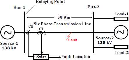
Singleline diagram of SPT line
When a single phase to ground fault occurs in multi phases at the same time at different locations is called a multi location phase to ground fault. As shown in figure 2, multi location phase to ground fault condition i.e, C-phase to ground (Cg) fault at 8 km and D-phase to ground (Dg) fault at 45 km with resistance (Rf) = 0 Ω and time = 40 ms are considered. As depicted in figure 2, fault current in D-phase is less than C-phase because fault current decreases with increase in fault location from sending end. When line to ground fault transforms to double line to ground fault after sometime interval at the same location is called a transforming phase to ground fault. Figure 3, explains transforming phase to ground fault that initially Cg fault at 8 km in 40 ms time is transformed after 10 ms to CDg fault at the same location. As illustrated in figure 3, fault current is same in C and D phases but fault occurring times are different. The recorded instantaneous six phase currents are fed to a 2nd low pass-butterworth filter (LP-BWF). The LP-BWF cut-off frequency is 480 Hz. After that, these currents are sampled with sampling frequency of 1.2 kHz. Then, signals are employed to one full cycle discrete fourier transform (DFT) for estimation of the fundamental components of six-phase current. Now these currents are normalized in between −1 to +1.
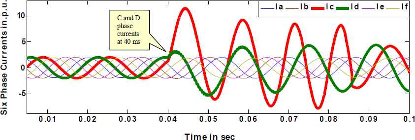
Six phase currents during multi location phase to ground fault
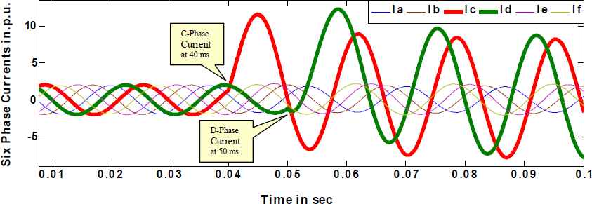
Six phase currents during transforming phase to ground fault
3. Procedure
FIS is employed for the proposed fault location method. FIS provides a nonlinear input and output mapping technique. It is an ideal platform for handling different problems with noisy and incomplete information. Fuzzy logic system contains four components: fuzzification, rule base, fuzzy inference engine and defuzzification. The rule base consists of rules which are extracted from expert knowledge to express nonlinear relationship between input domain and output domain. The rules are generally represented as IF-THEN statements. After that, the aggregation process which combines the output of each IF-THEN rule into only one fuzzy set. Then the outputs of aggregation are defuzzified into crisp values using the centroid method. The architecture of FIS is shown in figure 4. Designing of FIS consists of three major steps.
Step-1.Decide the number of inputs and outputs.
Step-2.Designing their membership functions (MFs)
Step-3.Implementing rules to connect inputs and outputs.

Outline of FIS architecture
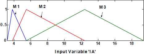
The framework of proposed FIS based location scheme for multi location and transforming phase to ground fault is illustrated in figure 5. The proposed fuzzy system is multi input-multi output system. Six inputs and six outputs are considered for FIS. The fundamental component of currents is fed into the FIS. Fault location in each phase is used as output. In this inputs represent IA, IB, IC, ID, IE and IF. The outputs represent La, Lb, Lc, Ld, Le and Lf. Mamdani FIS is applied to make decision. The non fuzzy values of inputs are converted into fuzzy degrees between 0 and 1 using triangular MFs. Each input has been separated into 3 partitions, viz. M1, M2 and M3 based on the location as depicted in figure 6. Similarly three groups of triangular MFs viz. DL1, DL2 and DL3 are designed for each output as illustrated in figure 7.In this M1<M2<M3 and DL1<DL2<DL3. After constructing input output fuzzy sets, IF-THEN fuzzy rules are formulated to evaluate the location of multi location and transforming phase to ground faults. FIS composed of total 729 rules. Some samples of IF-THEN rules are shown below.

Flow diagram of proposed work
- Rule1:
IF (I
a is M1) and (Ib is M1) and (Ic is M1) and (Id is M1) and (Ie is M1) and (If is M1)THEN (La is DL3) (Lb is DL3) (Lc is DL3) (Ld is DL3) (Le is DL3) (Lf is DL3)
- Rule2:
IF (I
a is M1) and (Ib is M1) and (Ic is M1) and (Id is M1) and (Ie is M1) and (If is M2)THEN (La is DL3) (Lb is DL3) (Lc is DL3) (Ld is DL3) (Le is DL3) (Lf is DL2)
- Rule3:
IF (I
a is M1) and (Ib is M1) and (Ic is M1) and (Id is M1) and (Ie is M1) and (If is M3)THEN (La is DL3) (Lb is DL3) (Lc is DL3) (Ld is DL3) (Le is DL3) (Lf is DL1)
- Rule4:
IF (I
a is M1) and (Ib is M1) and (Ic is M1) and (Id is M1) and (Ie is M2) and (If is M1)THEN (La is DL3) (Lb is DL3) (Lc is DL3) (Ld is DL3) (Le is DL2) (Lf is DL3)
- Rule5:
IF (I
a is M1) and (Ib is M1) and (Ic is M1) and (Id is M1) and (Ie is M2) and (If is M2)THEN (La is DL3) (Lb is DL3) (Lc is DL3) (Ld is DL3) (Le is DL2) (Lf is DL2)
- Rule6:
IF (I
a is M1) and (Ib is M1) and (Ic is M1) and (Id is M1) and (Ie is M2) and (If is M3)THEN (La is DL3) (Lb is DL3) (Lc is DL3) (Ld is DL3) (Le is DL2) (Lf is DL1)
- Rule7:
IF (I
a is M1) and (Ib is M1) and (Ic is M1) and (Id is M1) and (Ie is M3) and (If is M1)THEN (La is DL3) (Lb is DL3) (Lc is DL3) (Ld is DL3) (Le is DL1) (Lf is DL3)
- Rule8:
IF (I
a is M1) and (Ib is M1) and (Ic is M1) and (Id is M1) and (Ie is M3) and (If is M2)THEN (La is DL3) (Lb is DL3) (Lc is DL3) (Ld is DL3) (Le is DL1) (Lf is DL2)
- Rule9:
IF (I
a is M1) and (Ib is M1) and (Ic is M1) and (Id is M1) and (Ie is M3) and (If is M3)THEN (La is DL3) (Lb is DL3) (Lc is DL3) (Ld is DL3) (Le is DL1) (Lf is DL1)
- Rule10:
IF (I
a is M1) and (Ib is M1) and (Ic is M1) and (Id is M2) and (Ie is M1) and (If is M1)THEN (La is DL3) (Lb is DL3) (Lc is DL3) (Ld is DL2) (Le is DL3) (Lf is DL3)
·
·
- Rule27:
IF (I
a is M1) and (Ib is M1) and (Ic is M1) and (Id is M3) and (Ie is M3) and (If is M3)THEN (La is DL3) (Lb is DL3) (Lc is DL3) (Ld is DL1) (Le is DL1) (Lf is DL1)
- Rule28:
IF (I
a is M1) and (Ib is M1) and (Ic is M2) and (Id is M1) and (Ie is M1) and (If is M1)THEN (La is DL3) (Lb is DL3) (Lc is DL2) (Ld is DL3) (Le is DL3) (Lf is DL3)
·
·
- Rule81:
IF (I
a is M1) and (Ib is M1) and (Ic is M3) and (Id is M3) and (Ie is M3) and (If is M3)THEN (La is DL3) (Lb is DL3) (Lc is DL1) (Ld is DL1) (Le is DL1) (Lf is DL1)
- Rule82:
IF (I
a is M1) and (Ib is M2) and (Ic is M1) and (Id is M1) and (Ie is M1) and (If is M1)THEN (La is DL3) (Lb is DL2) (Lc is DL3) (Ld is DL3) (Le is DL3) (Lf is DL3)
·
·
- Rule243:
IF (I
a is M1) and (Ib is M3) and (Ic is M3) and (Id is M3) and (Ie is M3) and (If is M3)THEN (La is DL3) (Lb is DL1) (Lc is DL1) (Ld is DL1) (Le is DL1) (Lf is DL1)
- Rule244:
IF (I
a is M2) and (Ib is M1) and (Ic is M1) and (Id is M1) and (Ie is M1) and (If is M1)THEN (La is DL2) (Lb is DL3) (Lc is DL3) (Ld is DL3) (Le is DL3) (Lf is DL3)
·
·
- Rule729:
IF (I
a is M3) and (Ib is M3) and (Ic is M3) and (Id is M3) and (Ie is M3) and (If is M3)THEN (La is DL1) (Lb is DL1) (Lc is DL1) (Ld is DL1) (Le is DL1) (Lf is DL1)
Degree of MF for input of FIS
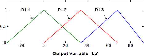
Degree of MF for output of FIS
After it combine the obtained outputs for each rule into a fuzzy set with a maximum fuzzy aggregation operator. The fuzzy set is then transformed into a numerical value by aggregating the consequents using centroid method to produce a non fuzzy value within 0 and 68. Now FIS is able to take the input currents and ready to locate multi location and transforming phase to ground faults.
4. Performance Evaluation
4.1. Multi location phase to ground faults
The proposed method is validated using data obtained from the MATLAB software. During healthy operating condition, all the six outputs are set to give the location value 67.5 < Location < 68 km. When the SPT line is subjected to multi location phase to ground fault at different locations in different phases then the outputs of corresponding faulty phases will give the different fault location values are in range of 0.5 < Location < 68 and healthy phase will be 68 km. The six outputs La, Lb, Lc, Ld, Le and Lf of the proposed method determine whether the fault is single location transforming phase to ground fault or multi location phase to ground fault. If any of the six outputs are in range of 0.5 < Location < 67.5 and the difference between corresponding phase estimated locations is greater than one then it is multi-location phase to ground fault. If any of the six outputs are in range of 0.5 < Location < 67.5 and the difference between corresponding phase estimated locations is less than one. Then the fault is treated as single location transforming phase to ground fault.
Most of phase to ground faults occurs without or with Rf. Majority of the fault location techniques are influenced by the Rf. Some of location techniques are not reliable due to the result of DC offset for variation in fault inception values. Therefore, it is important to study the performance of proposed technique for different fault inception values. In ordered to test the feasibility of the proposed mode, a large number of the multi location phase to ground fault studies corresponding wide variation of fault resistance (Rf = 35, 70 and 105 Ω) and fault inception angle (Ф=45, 90 and 135°). Table 1 presents the performance results of two location phase to ground faults for the different fault resistance and inception angles. Table 2 presents the performance results of three location phase to ground faults for the different fault resistance and inception angles. Table 3 presents the performance results of four location phase to ground faults for the different fault resistance and inception angles. Table 4 presents the performance results of five location phase to ground faults for the different fault resistance and inception angles. Table 5 presents the performance results of six location phase to ground faults for the different fault resistance and inception angles.
| Parameter | Rf (Ω) | Ф (°) | |||||
|---|---|---|---|---|---|---|---|
| Different values | 35 | 70 | 105 | 45 | 90 | 135 | |
| Two different location phase to ground faults | Ag at 22 km Bg at 15 km with Ф = 60° |
Ag at 18 km Dg at 13 km with Ф = 60° |
Bg at 62 km Dg at 9 km with Ф = 60° |
Eg at 61 km Fg at 41 km with Rf = 0 Ω |
Cg at 33 km Eg at 6 km with Rf = 0 Ω |
Ag at 55 km Fg at 17 km with Rf = 0 Ω |
|
| Phase A | La | 22.26 | 17.79 | 68 | 68 | 68 | 54.98 |
| Phase B | Lb | 15.12 | 68 | 61.89 | 68 | 68 | 68 |
| Phase C | Lc | 68 | 68 | 68 | 68 | 33.21 | 68 |
| Phase D | Ld | 68 | 13.03 | 9.14 | 68 | 68 | 68 |
| Phase E | Le | 68 | 68 | 68 | 61.17 | 5.85 | 68 |
| Phase F | Lf | 68 | 68 | 68 | 40.97 | 68 | 17.01 |
Test results of FIS for two different location phase to ground faults.
| Parameter | Rf (Ω) | Ф (°) | |||||
|---|---|---|---|---|---|---|---|
| Different values | 35 | 70 | 105 | 45 | 90 | 135 | |
| Three different location phase to ground faults | Ag at 46 km Cg at 8 km Eg at 33 km with Ф = 60° |
Cg at 27 km Dg at 13 km Fg at 66 km with Ф = 60° |
Bg at 3 km Dg at 43 km Eg at 53 km with Ф = 60° |
Dg at 60 km Eg at 5 km Fg at 2 km with Rf = 0 Ω |
Ag at 61 km Bg at 13 km Cg at 11 km with Rf = 0 Ω |
Bg at 19 km Eg at 27 km Fg at 37 km with Rf = 0 Ω |
|
| Phase A | La | 46.13 | 68 | 68 | 68 | 61.19 | 68 |
| Phase B | Lb | 68 | 68 | 2.71 | 68 | 12.82 | 19.01 |
| Phase C | Lc | 7.92 | 27.08 | 68 | 68 | 11.00 | 68 |
| Phase D | Ld | 68 | 12.90 | 43.13 | 59.83 | 68 | 68 |
| Phase E | Le | 33.24 | 68 | 53.16 | 5.18 | 68 | 27.13 |
| Phase F | Lf | 68 | 65.77 | 68 | 2.06 | 68 | 36.96 |
Test results of FIS for three different location phase to ground faults.
| Parameter | Rf (Ω) | Ф (°) | |||||
|---|---|---|---|---|---|---|---|
| Different values | 35 | 70 | 105 | 45 | 90 | 135 | |
| Four different location phase to ground faults | Ag at 5 km Dg at 42 km Eg at 31 km Fg at 14 km with Ф = 60° |
Bg at 24 km Dg at 25 km Eg at 18 km Fg at 1 km with Ф = 60° |
Cg at 11 km Dg at 35 km Eg at 44 km Fg at 15 km with Ф = 60° |
Bg at 58 km Cg at 21 km Dg at 9 km Eg at 17 km with Rf = 0 Ω |
Ag at 33 km Bg at 16 km Cg at 19 km Dg at 47 km with Rf = 0 Ω |
Ag at 8 km Bg at 50 km Cg at 23 km Fg at 13 km with Rf = 0 Ω |
|
| Phase A | La | 4.91 | 68 | 68 | 68 | 32.78 | 7.76 |
| Phase B | Lb | 68 | 24.11 | 68 | 58.04 | 16.16 | 49.89 |
| Phase C | Lc | 68 | 68 | 10.94 | 20.98 | 19.27 | 23.13 |
| Phase D | Ld | 42.32 | 25.24 | 35.16 | 9.14 | 46.72 | 68 |
| Phase E | Le | 31.30 | 18.15 | 43.80 | 17.09 | 68 | 68 |
| Phase F | Lf | 14.25 | 0.69 | 15.21 | 68 | 68 | 12.75 |
Test results of FIS for four different location phase to ground faults.
| Parameter | Rf (Ω) | Ф (°) | |||||
|---|---|---|---|---|---|---|---|
| Different values | 35 | 70 | 105 | 45 | 90 | 135 | |
| Five different location phase to ground faults | Ag at 16 km Bg at 10 km Cg at 61 km Dg at 15 km Eg at 53 km with Ф = 60° |
Ag at 63 km Bg at 28 km Cg at 9 km Dg at 13 km Fg at 65 km with Ф = 60° |
Ag at 25 km Bg at 34 km Cg at 51 km Eg at 30 km Fg at 7 km with Ф = 60° |
Ag at 35 km Bg at 1 km Dg at 43 km Eg at 6 km Fg at 56 km with Rf = 0 Ω |
Ag at 9 km Cg at 13 km Dg at 40 km Eg at 24 km Fg at 32 km with Rf = 0 Ω |
Bg at 36 km Cg at 48 km Dg at 21 km Eg at 26 km Fg at 11 km with Rf = 0 Ω |
|
| Phase A | La | 16.23 | 63.18 | 24.81 | 34.83 | 9.33 | 68 |
| Phase B | Lb | 10.32 | 27.86 | 34.00 | 0.94 | 68 | 36.15 |
| Phase C | Lc | 60.91 | 8.83 | 51.22 | 68 | 13.06 | 48.24 |
| Phase D | Ld | 15.11 | 12.86 | 68 | 42.97 | 40.19 | 21.06 |
| Phase E | Le | 52.97 | 68 | 30.16 | 5.74 | 23.85 | 25.96 |
| Phase F | Lf | 68 | 64.70 | 7.27 | 56.05 | 32.23 | 11.05 |
Test results of FIS for five different location phase to ground faults.
| Parameter | Rf (Ω) | Ф (°) | |||||
|---|---|---|---|---|---|---|---|
| Different values | 35 | 70 | 105 | 45 | 90 | 135 | |
| Six different locationphase to ground faults | Ag at 12 km Bg at 6 km Cg at 35 km Dg at 21 km Eg at 16 km Fg at 13 km with Ф = 60° |
Ag at 63 km Bg at 21 km Cg at 39 km Dg at 34 km Eg at 51 km Fg at 67 km with Ф = 60° |
Ag at 16 km Bg at 15 km Cg at 54 km Dg at 31 km Eg at 61 km Fg at 6 km with Ф = 60° |
Ag at 18 km Bg at 1 km Cg at 26 km Dg at 24 km Eg at 65 km Fg at 38 km with Rf = 0 Ω |
Ag at 61 km Bg at 12 km Cg at 4 km Dg at 55 km Eg at 9 km Fg at 37 km with Rf = 0 Ω |
Ag at 48 km Bg at 13 km Cg at 52 km Dg at 7 km Eg at 14 km Fg at 19 km with Rf = 0 Ω |
|
| Phase A | La | 12.03 | 63.11 | 15.74 | 18.16 | 61.24 | 48.14 |
| Phase B | Lb | 6.29 | 21.30 | 15.11 | 1.25 | 12.23 | 13.10 |
| Phase C | Lc | 34.96 | 39.22 | 54.03 | 26.12 | 4.31 | 52.29 |
| Phase D | Ld | 21.19 | 34.21 | 31.18 | 23.86 | 55.3 | 7.13 |
| Phase E | Le | 15.87 | 51.02 | 61.11 | 65.23 | 8.85 | 13.84 |
| Phase F | Lf | 13.22 | 67.10 | 6.21 | 38.06 | 36.98 | 19.12 |
Test results of FIS for six different location phase to ground faults.
One sample of result for multi location phase to ground faults in MATLAB fuzzy software is given in figure 8. This result was obtained when C-phase to ground (Cg) fault at 20 km and E-phase to ground (Eg) fault at 40 km with Rf = 0 Ω and time = 40 ms are considered. It can be observed here that faults are classified with the help of location results without classification technique. It also classifies and locates all types of phase to ground faults. Figure 9, illustrates the outputs of fault classification FIS in which ‘C’ phase goes 20 km at 40 ms and E goes 40 km at 40 ms, with other outputs A,B,D and F remaining high (68 km) showing there is CEg-multi location phase to ground fault.
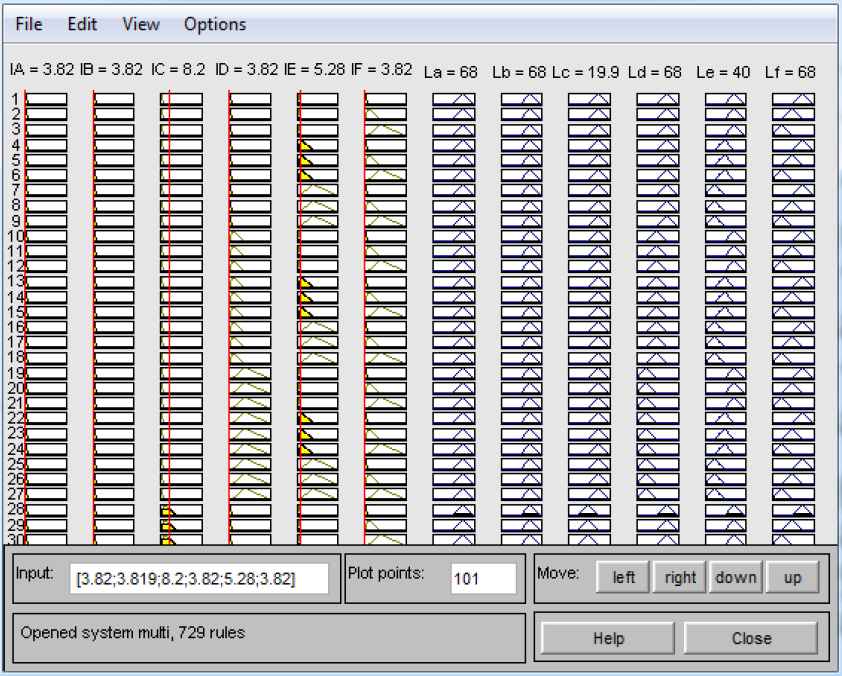
Evaluation view of FIS output in case of multi location faults
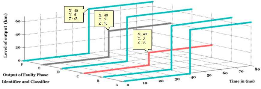
Classification view of FIS output in case of multi location faults
4.2. Transforming phase to ground faults
In addition to multi location phase to ground faults, transforming phase to ground faults also occur in SPT line. When the SPT line is subjected to transforming phase to ground fault at same location in different phases then the output of corresponding faulty phases will give the same fault location values are in range of 0.5 < Location < 68 and healthy phase will be 68 km. The proposed system is able to locate not only multi location phase to ground faults, but also transforming phase to ground faults. The proposed FIS method has been evaluated for around 1000 fault simulation cases and has been carried out under transforming faults with varying parameters such as fault location, fault resistance and fault inception angle. The performance results obtained by the proposed method for transforming faults based on fuzzy are summarized in table 6–10.
| Parameter | Rf (Ω) | Ф (°) | |||||
|---|---|---|---|---|---|---|---|
| Different values | 35 | 70 | 105 | 45 | 90 | 135 | |
| 1 phase to ground transformed to other phases | Eg to EFg at 8 km with Ф = 60° | Cg to CDEg at 17 km with Ф = 60° | Ag to ABCDg at 54 km with Ф = 60° | Bg to BCg at 66 km with Rf=0 Ω | Ag to ABCDEg at 22 km with Rf= 0Ω | Ag to ABCDEFg at 12 km with Rf =0 Ω | |
| Phase A | La | 68 | 68 | 54.34 | 68 | 22.01 | 12.03 |
| Phase B | Lb | 68 | 68 | 53.99 | 65.88 | 21.93 | 12.12 |
| Phase C | Lc | 68 | 17.32 | 54.16 | 65.80 | 22.03 | 12.05 |
| Phase D | Ld | 68 | 17.05 | 54.06 | 68 | 22.06 | 12.05 |
| Phase E | Le | 8.02 | 16.86 | 68 | 68 | 22.10 | 12.09 |
| Phase F | Lf | 8.09 | 68 | 68 | 68 | 68 | 12.00 |
Test results of FIS for single phase to ground fault transformed to other phase to ground faults.
| Parameter | Rf (Ω) | Ф (°) | |||||
|---|---|---|---|---|---|---|---|
| Different values | 35 | 70 | 105 | 45 | 90 | 135 | |
| 2 phase to ground transformed to other phases | BCg to BCDg at 29 km with Ф = 60° | CDg to CDEFg at 18 km with Ф = 60° | ABg to ABCDEg at 32 km with Ф = 60° | DEg to DEFg at 24 km with Rf=0 Ω | ABg to ABCDFg at 67 km with Rf=0 Ω | ABg to ABCDEFg at 48 km with Rf=0 Ω | |
| Phase A | La | 68 | 68 | 31.93 | 68 | 67.23 | 48.02 |
| Phase B | Lb | 29.19 | 68 | 32.00 | 68 | 67.31 | 48.25 |
| Phase C | Lc | 29.23 | 18.03 | 32.06 | 68 | 67.04 | 48.12 |
| Phase D | Ld | 28.85 | 17.85 | 31.87 | 23.79 | 66.85 | 48.08 |
| Phase E | Le | 68 | 17.98 | 31.99 | 24.08 | 68 | 48.03 |
| Phase F | Lf | 68 | 17.96 | 68 | 24.17 | 66.83 | 47.76 |
Test results of FIS for two phase to ground fault transformed to other phase to ground faults.
| Parameter | Rf (Ω) | Ф (°) | |||||
|---|---|---|---|---|---|---|---|
| Different values | 35 | 70 | 105 | 45 | 90 | 135 | |
| 3 phase to ground transformed to other phases | ABCg to ABCDg at 14 km with Ф = 60° | ABCg to ABCDEg at 11km with Ф = 60° | ABCg to ABCDEFg at 36 km with Ф = 60° | ABCg to ABCDg at 21 km with Rf=0 Ω | ABCg to ABCDEg at 24 km with Rf=0 Ω | ABCg to ABCDEFg at 38 km with Rf=0 Ω | |
| Phase A | La | 13.89 | 10.97 | 36.22 | 21.03 | 24.05 | 38.09 |
| Phase B | Lb | 13.80 | 11.04 | 35.99 | 20.95 | 24.13 | 38.15 |
| Phase C | Lc | 14.21 | 11.05 | 36.21 | 21.24 | 24.32 | 38.23 |
| Phase D | Ld | 14.05 | 11.23 | 36.02 | 21.08 | 24.31 | 37.98 |
| Phase E | Le | 68 | 10.88 | 36.03 | 68 | 24.06 | 37.77 |
| Phase F | Lf | 68 | 68 | 36.08 | 68 | 68 | 38.08 |
Test results of FIS for three phase to ground fault transformed to other phase to ground faults.
| Parameter | Rf (Ω) | Ф (°) | |||||
|---|---|---|---|---|---|---|---|
| Different values | 35 | 70 | 105 | 45 | 90 | 135 | |
| 4 phase to ground transformed to other phases | ABCDg to ABCDEg at 21 km with Ф = 60° | ABCDg to ABCDEg at 58 km with Ф = 60° | ABCDg to ABCDEg at 52 km with Ф = 60° | ABCDg to ABCDFg at 16 km with Rf=0 Ω | ABCDg to ABCDFg at 31 km with Rf=0 Ω | ABCDg to ABCDFg at 15 km with Rf=0 Ω | |
| Phase A | La | 21.13 | 58.21 | 51.75 | 16.25 | 31.02 | 15.11 |
| Phase B | Lb | 21.07 | 58.19 | 51.69 | 16.33 | 31.24 | 15.06 |
| Phase C | Lc | 21.33 | 58.22 | 52.02 | 16.33 | 31.34 | 14.96 |
| Phase D | Ld | 21.21 | 58.15 | 52.20 | 16.15 | 31.20 | 15.32 |
| Phase E | Le | 21.33 | 58.21 | 52.10 | 68 | 68 | 68 |
| Phase F | Lf | 68 | 68 | 68 | 16.04 | 31.07 | 15.16 |
Test results of FIS for four pase to ground fault transformed to other phase to ground faults.
| Parameter | Rf (Ω) | Ф (°) | |||||
|---|---|---|---|---|---|---|---|
| Different values | 35 | 70 | 105 | 45 | 90 | 135 | |
| 5 phase to ground transformed to other phases | ABCDEg to ABCDEFg at 63 km with Ф = 60° | ABCDEg to ABCDEFg at 55 km with Ф = 60° | ABCDEg to ABCDEFg at 5 km with Ф = 60° | ABCDEg to ABCDEFg at 33 km with Rf=0 Ω | ABCDEg to ABCDEFg at 9 km with Rf=0 Ω | ABCDEg to ABCDEFg at 15 km with Rf=0 Ω | |
| Phase A | La | 63.12 | 55.01 | 5.09 | 33.11 | 9.02 | 15.06 |
| Phase B | Lb | 63.15 | 54.96 | 5.11 | 33.08 | 9.16 | 14.92 |
| Phase C | Lc | 63.03 | 55.05 | 5.13 | 33.00 | 9.21 | 15.03 |
| Phase D | Ld | 63.11 | 55.06 | 5.07 | 32.80 | 9.02 | 15.08 |
| Phase E | Le | 63.02 | 55.00 | 5.07 | 33.01 | 9.11 | 15.12 |
| Phase F | Lf | 63.23 | 55.05 | 5.10 | 33.01 | 9.07 | 15.01 |
Test results of FIS for five phase to ground fault transformed to other phase to ground faults.
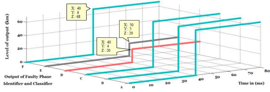
One sample of result for transforming phase to ground faults in MATLAB fuzzy software is given in figure 10. Figure 11, depicts the outputs of fault classification FIS in which ‘D’ phase goes 20 km at 40 ms and E goes 20 km at 50 ms, with other outputs A,B,C and F remaining high (68 km) showing there is DEg-transforming phase to ground fault. It can be found that most of the test cases can be located with 0.34 km difference.
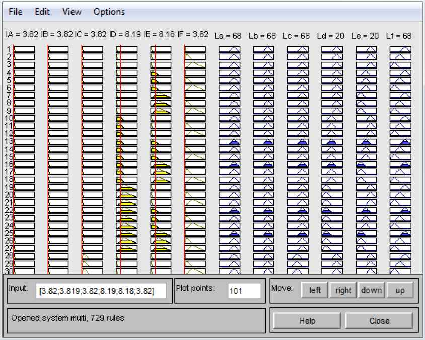
Evaluation view of FIS output in case of transforming faults
Classification view of FIS output in case of transforming faults
4.3. Comparison with other techniques
To judge the expediency of the technique, the comparison study has been carried out for maximum deference between actual and measured value of fault location and technique used. The proposed technique has been compared with the test results reported in Ref 22, 23, 30. The comparison of proposed technique with established methods are shown in table 11. The maximum deference between actual and measured value of fault location estimation in Ref 22, 23 are 0.459 km and 0.468 km respectively. As revealed from the simulation results, the proposed method raised accurate performance for multi location and transforming phase to ground faults with the maximum deference between actual and measured value of fault location estimation levels of 0.30 km and 0.34 km for both cases, respectively. Distance estimation method 30 for multi location and transforming faults is also developed using ANN. The drawback of the ANN based approach is that it requires training process which requires bulky training samples, training algorithms, number of hidden layers, choice of the transfer function, neurons, epochs and setting goal. It is noteworthy to mention that the FIS does not employ large number of training samples however it performs very well and correctly.
| Reference no | 22 | 23 | 30 | Proposed method |
|---|---|---|---|---|
| Inputs used | Voltages and currents | Voltages and currents | Voltages and currents | Only currents |
| Transmission line type | SPT line | SPT line | Three phase transmission line | SPT line |
| Fault type | Shunt faults | Shunt faults | Multi location and transforming faults | Multi location and transforming faults |
| Protection function | Fault zone identification and location | Fault detection, classification and location | Fault location | Fault location |
| Algorithm used | Modular neuro wavelet | Wavelet and artificial neural networks | Artificial neural networks | FIS |
| Maximum difference of actual and measured value | 0.459 km | 0.468 km | 1 km | 0.34 km |
Comparison of the proposed technique with established methods
5. Conclusion
A precise fault location method for SPT lines was proposed using FIS and single end currents. DFT is used for pre-processing of the six phase current signals. The fundamental component of currents has been only employed by taking into account for proposed method. The proposed approach does not require any classification method for phase to ground faults classification. Also, the method is independent of the receiving end data. FIS with IF-THEN rules has been arranged for fault location estimation. This facilitated locating all multi location phase to ground fault types including transforming faults successfully. Evaluation studies have discussed that the proposed method can yield accurate estimates under variety of fault conditions for SPT line. In addition, the maximum deference between actual and measured value of fault location does not exceed 0.34 km in all test cases. The suggested technique based on fuzzy for fault location is promising solution compared with earlier techniques and the test results verify the superiority of the proposed fuzzy based scheme over other schemes for fault location.
Appendix A.
| Parameter | Units | Values |
|---|---|---|
| Number of Circuits | - | 1 |
| Number of Phases | - | 6 |
| Source Voltage | [kV] | 138 |
| Base Voltage | [kV] | 138 |
| Base Power | [MVA] | 100 |
| Frequency | [Hz] | 60 |
| Earth Resistivity | [Ω-m] | 100 |
| Line Length | [km] | 68 |
| Short Circuit Capacity | [MVA] | 1250 |
| Source X/R Ratio | - | 10 |
| [kW] | 100 | |
| Load at Bus | [kVAR] | 100 |
References
Cite this article
TY  - JOUR
AU  - A Naresh Kumar
AU  - M Chakravarthy
PY  - 2018
DA  - 2018/03/16
TI  - Fuzzy Inference System Based Distance Estimation Approach for Multi Location and Transforming Phase to Ground Faults in Six Phase Transmission Line
JO  - International Journal of Computational Intelligence Systems
SP  - 757
EP  - 769
VL  - 11
IS  - 1
SN  - 1875-6883
UR  - https://doi.org/10.2991/ijcis.11.1.58
DO  - 10.2991/ijcis.11.1.58
ID  - Kumar2018
ER  -