
ABC and DE Algorithms based Fuzzy Modeling of Flight Data for Speed and Fuel Computation
- DOI
- 10.2991/ijcis.11.1.60How to use a DOI?
- Keywords
- fuzzy modeling; fuzzy rule design; artificial bee colony algorithm; flight control system
- Abstract
It is crucial to evaluate the information obtained from the sensors in a fast and accurate manner in air vehicles exposed to many internal and external influences during their flights. The effectiveness and flexibility of the reasoning method comes to the forefront when the pilot or flight control system makes the necessary decisions in critical situations. The method used should be able to provide the nearest response to the decision that the pilot has to give, even when working with complex, unclear or incomplete data. Thus, it is not the correct approach to think that sensorial measurements and methods that describe them through a model are separate from each other. In this study, a fuzzy rule based model is designed using some important measurement data belonging to a flight control system for simultaneously computation of speed and fuel parameters. The fuzzy model parameters are determined by using artificial bee colony (ABC) and differential evolution (DE) algorithms in the modeling process in which actual flight data of Boeing B-767-200ER type aircraft are used. To demonstrate the efficiency of the modeling approach and the algorithms, fuzzy model structures having 3 inputs-and-2 outputs for different rule numbers are tested. The inputs of the fuzzy models are considered as altitude, weight, and engine pressure ratio. On the other hand, parameters of the flight speed and fuel amount are used for outputs of the models. The results achieved from the models are comparatively presented with each other and actual values.
- Copyright
- © 2018, the Authors. Published by Atlantis Press.
- Open Access
- This is an open access article under the CC BY-NC license (http://creativecommons.org/licences/by-nc/4.0/).
1. Introduction
Flight control systems play a crucial role in ensuring the management of aircrafts navigation which consists of takeoff, straight flight and landing stages in general. In order to ensure a safe and comfortable flight, a great number of vital measurements, evaluations, calculations and planning must be made simultaneously by considering many factors inside and outside the aircraft1–7. At this stage, the accuracy of sensorial measurements and their rapid evaluation by the pilot are key priorities for flight safety. For this purpose, management of the flight control system and equipment placed in the aircraft should not be difficult and complicated for pilots. In fact, these systems should be able to support pilots even in the presence of inadequate and/or uncertain measurement information.
The altitude at the time of flight, the weight of the aircraft, engine pressure ratio (EPR) which is the ratio of the turbine discharge pressure divided by the compressor inlet pressure, the current speed and amount of fuel consumed play a major role in determining the duration of the flight. Two of the most important factors affecting the flight time and its safety are the parameters of speed and fuel amount. According to the changing conditions over time, by evaluating some flight-related information fastly and accurately, the speed and fuel information should be calculated and delivered to the pilot as soon as possible.
This study focuses on calculating the optimal speed and the fuel amount according to three important flight parameters of an aircraft, namely, the flight altitude, aircraft weight, and EPR value. For the calculation using data from Boeing’s B-767-200ER aircrafts, fuzzy model structures with 3 inputs and 2 outputs are proposed. Parameters of the fuzzy models are optimized by using artificial bee colony (ABC) and differential evolution (DE) algorithms. Several successful fuzzy modeling studies based on the use of artificial intelligence algorithms are available in the literature8–17. Genetic algorithm is used to obtain Takagi-Sugeno type fuzzy model structure in the study presented by Siarry and Guely8. In the study given by Kang et.al, an evolutionary programming approach to determine the fuzzy rule structure and model parameters is used in nonlinear system modeling and control process9. A study involving the approach of obtaining a fuzzy rule set based on the particle swarm optimization (PSO) method using an existing input-output data set is presented by Chen10. In the mentioned study, recursive least squares method is also applied in finding the consequent parameters of the fuzzy system. A useful study is presented by Bagis11, which involves determining the parameters of the fuzzy rule based systems by the tabu search algorithm (TSA) for nonlinear system modeling. In other research given by Habbi et.al14, an ABC algorithm based methodology to automatically obtain Takagi-Sugeno type fuzzy systems is proposed. Investigation reported by Konar and Bagis15 presents a detailed performance comparison of PSO, DE and ABC algorithms to determine the parameters of the fuzzy models. The parameters of the single-output fuzzy models proposed in the mentioned study, examining the Box-Jenkins gas furnace problem and the antenna modeling problem, are obtained based on the use of mean squared error (MSE) performance index. To define a measured data set obtained from an optical sensing circuit for glucose detection, ABC algorithm based 3 inputs-1 output fuzzy models are used by Saracoglu et.al17.
Several studies on modeling and simulation of flight control systems are included in the literature18–34. In the study by Góes et.al18, a comparison of two output-error methods to inverse modeling of an aircraft are presented by using the experimental flight data. The paper given by Sembiring et.al21 deals with the estimation of unmeasured parameters based on flight data recorded in quick access recorder (QAR) device. In the paper, the purpose of estimating the selected parameters such as wind speed component, time-history based of lift and drag coefficient, drag due to spoiler deflection, friction coefficients and thrust during the ground run phase is explained as a benefit that can be obtained in aircraft incident/accident investigation. An overview of existing methods about aircraft performance monitoring from flight data is presented by Krajček et.al22. On the other hand, a method for identifying maneuver type from operational flight data is proposed by analyzing the flight attitude of aircraft23. In the study presented by Notter et.al25, a mathematical model for the coupled system dynamics of a multirotor unmanned aerial vehicle with heavy slung load is derived. The study given by Goupil et.al26 presents signal processing strategy based a data driven approach for the detection of failures impacting the flight control system. To estimate all possible aircraft touchdown attitudes and control inputs based on flight dynamics simulations and Monte Carlo evaluation, a solution is proposed by Wu et.al27. The other solution proposal of Alcalay et.al28 for estimation of flight parameters in nominal and degraded flight conditions is based on virtual sensors which make use of an adaptive extended Kalman filter. However, a neural network based adaptive flight control system which is able to compensate the system uncertainties, adapt to the changes in flight conditions, and accommodate the system failures is described in the study given by Savran et.al30 In order to enhance the reliability of flight control systems, another neural network based direct adaptive fault tolerance control approach is proposed by Xiaoxiong et.al31 Similarly, a fuzzy logic modeling method based on flight data to illustrate the prediction of the factors contributing to the degradation of aerodynamic efficiency in flight operations is presented by Chang33. In the study of Roy and Peyada34, adaptive neuro-fuzzy system and artificial bee colony algorithm are employed to model and estimate the nonlinear characteristics of an aircraft.
On the other hand, in our previous studies on this subject, the flight speed and fuel amount information during takeoff and climbing of the Boeing’s B-737-300 type aircrafts are obtained by using Anfis (Adaptive network based fuzzy inference system) and neural network models5,6. In our other study, Anfis and neural models are presented for simultaneous computation of the speed and fuel parameters of Boeing’s B-767-200ER type aircrafts7.
The main purpose of this study is to provide an optimized model structure for simultaneously computation of some critical parameters of a flight control system in the aircraft. The three factors came together for the first time in this study for a common purpose: simultaneously determination of speed and fuel flight parameters by evaluating different flight parameters, the use of a multi input-multi output fuzzy model structure for this purpose, and the employ of ABC and DE algorithms in the fuzzy model optimization. This attempt demonstrates the innovation and contribution in this study when compared to the other studies in the literature.
One of the main motivations of this study is to investigate the performance of the multi-input and multi-output fuzzy modeling in a flight control system. Furthermore, this paper interrogates and compares the capabilities of the ABC and DE algorithms to determine the parameters of the fuzzy models with different rule numbers.
The remainder of this paper is organized as follows. In the next section, the basic properties of the ABC and DE algorithms are introduced briefly. The modeling problem and fuzzy model structures used are provided in Section 3. Section 4 presents the results of the fuzzy models optimized by the algorithms. Finally, some concluding remarks are made in the last section.
2. Algorithms used in this study
2.1. ABC Algorithm
ABC algorithm introduced by Karaboga is a population-based method which provides impressive solutions especially for numerical optimization problems35–37. The basic principle of this method is based on the definition of the food search behavior of three grouped bee colonies. The location of food resources represents a possible solution to the problem. The food sources (solutions) and their neighbors (new solutions) are determined by the employed bees. The amount of nectar in the sources indicates the qualities of the solutions and is defined as the fitness function. Evaluation of this information and selection of the new possible food sources depending on the nectar amounts is achieved by the onlooker bees. The procedure for selecting new possible sources is carried out by scout bees and the “limit” parameter is used for this. According to this parameter which defines the predetermined number of cycles, if a solution cannot be improved by a selected limit value, then the related food source is abandoned by the algorithm. During the search procedure, the best food sources with high quality found so far are retained in the memory. These steps for the entire “colony size (CS)” are repeated until a specific stopping criteria, for instance during the number of “maximum cycles”, is satisfied, and the quality of the solutions is progressively improved by the algorithm.
The main steps of the ABC algorithm can be summarized as the following36:
- (1)
Initialize population
- (2)
Repeat the following steps until the stopping criterion is satisfied
- (3)
Send the employed bees to the food sources
- (4)
Send the onlooker bees to the food sources according to nectar amounts (calculation of the fitness values)
- (5)
Send the scout bees in order to find the new sources (determination of the limit values)
- (6)
Memorize the best food source found so far
- (7)
If stopping criterion is not met, go back to step 3.
The algorithm usually uses a mathematical definition as follows to discover new solutions:
This description dispatches the research to a new possible food source Vij that is of better quality than a source in the position i. In here, k (k ∈ {1,2,…..,pop_size}) is a randomly chosen index, Xij and Xkj are current and neighbor solutions, respectively. In this paper, the limit value is performed according to the definition of [(colony size÷2) × number of the parameters].
2.2. DE Algorithm
DE algorithm (DEA) is a simple population based evolutionary algorithm presented by Storn and Price for minimizing possibly nonlinear and non-differentiable type functions38,39. In the algorithm that uses basic operations such as mutation, crossover and selection, the differences between solution elements randomly determined are used to obtain new solutions. In this process called mutation, the differences between solution elements are weighted and added to another solution element to obtain solution diversity. The general form of such an operation can be given as follows16,40:
In these equations, Vi,j,G+1 is the new (mutant) vector, randj is a uniform random number in range of [0,1], CR is the crossover rate (CR ∈ [0, 1]), j is an integer number (j =1, 2, .., D), D is number of the variables, and jrand is a random number in [1,D].
Because of our experience with our previous work, the control parameters for the algorithms in this study have been determined as follows: For the ABC algorithm, CS=30 and 40, limit value= (CS/2) × (optimized parameter number); for the DEA, population size=30 and 40, crossover rate=0.9, scaling factor (F)=0.8. Each algorithm-based modeling study was repeated at least 30 times for 5000 iterations, and the best results are presented here.
3. Definition of the Problem and Fuzzy Rule Based Model used in This Study
3.1. Flight Data
In the present study, the flight data in the operation manual of Boeing B767-200 aircraft document is employed for modeling process3. According to this document, the 767 airplane family that provides maximum market versatility is the most widely used across the Atlantic. This 767 family has four models commonly used, including 767-200ER (extended-range), 767-300ER, 767-300 Freighter and 767-400ER. The main technical specifications of the Boeing B767-200ER aircraft used in this study are as follows3: length=159 feet 2 inches, wingspan=156 feet 1 inches, tail height=52 feet, engines= Pratt & Whitney PW 4000, basic maximum takeoff weight=345.000 pounds, fuel capacity=24.140 U.S. gallons, maximum range=6.650 Nm, altitude capability=37.900 feet, cruise speed= Mach 0.80 (530 mph), cargo capacity=3.070 cubic feet.
For the modeling, the data set in the two engine holding speeds and fuel flow table of the aircraft document mentioned above is used. This data set is in the form of an information matrix that includes the altitude (feet), gross weight (1000 pounds), engine pressure ratio (EPR), speed (KIAS, knots-indicated air speed) and fuel flow (lb/hr) values of the aircraft. The upper and lower bounds of these parameters are indicated as follows in the table, respectively: [1500–40000] feet, [210–310] (1000 pounds), [1.01–1.51], [200–232] knots, [6580–10620] lbs/hr.
3.2. Fuzzy Model Structure for Flight Data
In the operational manual document of the aircraft considered in this study, measurement information about speeds and fuel flow at different altitude, weight and EPR values for the aircraft is included. This speed-fuel table is limited to 80 data sets, and does not provide information about intermediate values. If the current data set can be defined well with a model, intermediate (unmeasured) values that are not included in the table can also be obtained. In fact, the main purpose of the model is to find the values that are closest to the speed and fuel data that would have been obtained if more real-time (actual) measurements had been made. These values obtained by using a model that is optimized by an algorithm in general are named as optimal values. Thus, using the flight parameters generated by the model when necessary, more confident and accurate decisions can be made for flight safety. One of the fast and most effective methods that can be used for this purpose is the fuzzy modeling approach11,16,17,41.
The essence of the problem is to estimate the most accurate speed and fuel consumption values simultaneously with the help of a model, depending on some input information measured during the flat flights of the aircrafts. For this purpose, a fuzzy model structure using the altitude (A, feet), gross weight (W, 1000 pound) and EPR values of Boeing B-767-200ER aircraft as input information is taken into consideration3,7. The most a ccurate speed (S, knot=nautical mile/hour) and fuel (F, lb/h) information to be obtained is taken as the outputs of the model. Thus, the model examined in this study is introduced to describe a 3-input and 2-output system (Figure 1).

Fuzzy model structure used in the study
For modeling the multi-input multi-output system, the fuzzy model structure presented by Bagis is preferred11,16,17,41. In this model structure called as “singleton model”, the reasoning procedure is provided by multiplying the weighted input membership functions and the output singleton values. The main difference of this study from the others is that this fuzzy logic based model structure is applied for the first time to the flight control system data, which is one of the difficult modeling problems. Moreover, the fuzzy model is dual-output and instead of the typical MSE error in determining the model parameters, the performance index (PI) value, which is described below, is used. The features mentioned constitute the fundamental differences that distinguish this work from the others and the basic contribution of this work. Figure 2 shows the singleton fuzzy inference system (FIS) for a system of 2 rules with 3 inputs and 2 outputs.

Fuzzy inference mechanism used in this study
From Figure 2, it is observed that the triangular and singleton type membership functions are used to define the inputs and outputs, respectively. Thus, the number of parameters required to define a rule is 14 as shown in Table 1. When the number of rules is 5, 10, and 16, the number of required parameters will be 70, 140, and 224, respectively. The main task expected from the algorithms is to determine these parameters at the optimum values.
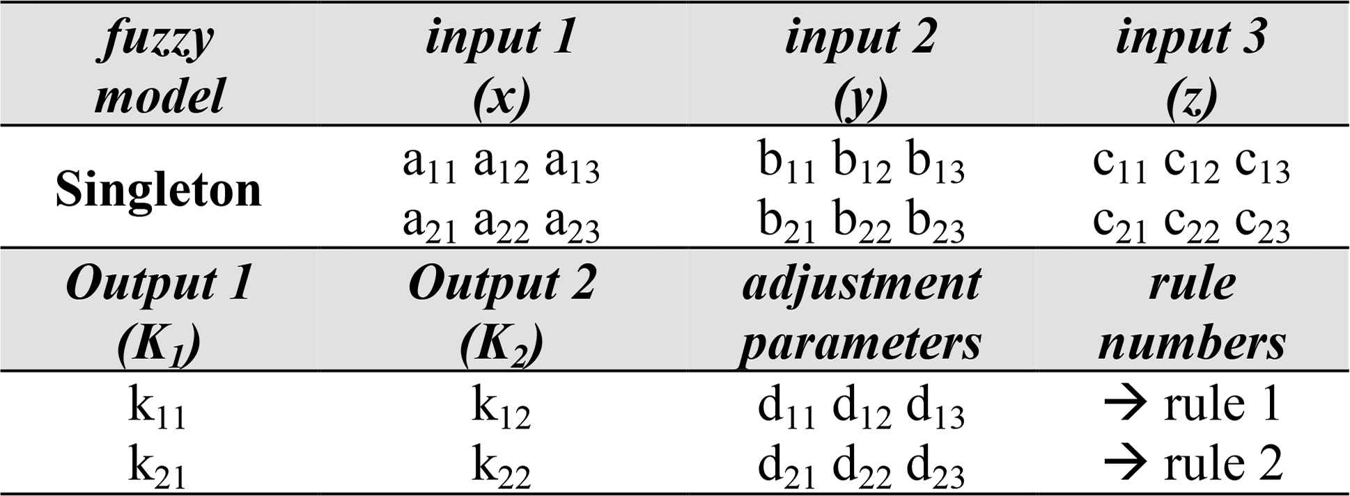
Definition of the parameters in a singleton fuzzy model with two rules
As can be seen from the definition in Table 1, there is no mathematical expression for the fuzzy model structure used in this study. Instead, the fuzzy model structure is defined by a parameter matrix that specifies the rules. Accordingly, there are 14 parameters in each rule line. The first nine parameters are used to define triangular membership functions composed for 3 inputs (A, W and EPR). The 10th and 11th parameters are singleton values for speed (S) and fuel (F) outputs. The last three values are the adjustment parameters used to calculate each output.
Thus, the ith fuzzy rule structure can be expressed by a general form such as
Similar calculations are made for other variables.
In order to increase modeling effectiveness, while the normalization intervals for the input variables A, W and EPR used in the presented system model are [500, 50000], [200, 350], [0.8, 2] respectively, the normalization intervals for the S and F output variables are [180, 250] and [6000, 11000], respectively again.
The K1* and K2* notations in the Figure 2 describe the fuzzy reasoning mechanism. These notations are used for speed (S) and fuel (F) respectively. In here, µ(x), µ(y) and µ(z) are the membership values for x (A), y (W) and z (EPR) inputs.
To evaluate the performance of the fuzzy models with different rule numbers, a performance indicator, shown as PI, is used11,42,43. In the definition given as Equation 7,
After several trials, it was seen that mean squared error (MSE) based studies did not provide the desired success when the fuzzy model has two outputs. In fuzzy models that are optimized by considering MSE, it was observed that the error value of two outputs cannot be reduced simultaneously in the desired form. Therefore, in this study, it was tried to find the best model parameters considering the minimization of the PI values of the models. However, the MSE values of the models in the results tables are also noted. In the simulations, the Matlab® programming package and Intel Pentium 2800MHz computers are used44,45.
4. Results of the Fuzzy Models and Discussion
In this modeling study having models with different rule numbers such as 2, 3, 4, 5, 7, 8, 10 and 16, 73 train and 7 test data are used by the algorithms3,41. To obtain the model parameters, two different population (or colony) sizes such as 30 and 40 are tested for different fuzzy rule base structures with different number of model parameters. The best PI values of the fuzzy models obtained by the ABC and DE algorithms are presented in Table 2 and Table 3. While the results in Table 2 are given for 30 CS, the values in Table 3 are of a CS of 40.
| Rules | Algorithm | MSE (CS=30) | PI | |||
|---|---|---|---|---|---|---|
| Speed | Fuel | |||||
| Train | Test | Train (e+003) | Test (e+003) | |||
| 2 | ABC | 9.0073 | 6.1290 | 6.4252 | 12.253 | 0.0028 |
| DE | 8.9424 | 4.7931 | 8.2826 | 6.9358 | 0.0029 | |
| 3 | ABC | 0.6422 | 0.8480 | 7.0396 | 4.9606 | 0.0016 |
| DE | 1.0220 | 0.6774 | 3.0875 | 2.7636 | 0.0013 | |
| 4 | ABC | 0.5380 | 0.6002 | 5.0293 | 5.3442 | 0.0014 |
| DE | 0.7015 | 0.3446 | 3.0741 | 2.6144 | 0.0012 | |
| 5 | ABC | 0.3858 | 0.3280 | 4.4451 | 4.2444 | 0.0013 |
| DE | 0.6245 | 1.3180 | 3.6455 | 1.7345 | 0.0013 | |
| 7 | ABC | 0.5482 | 0.8548 | 3.1175 | 4.1769 | 0.0012 |
| DE | 0.4056 | 0.4411 | 3.8047 | 3.3118 | 0.0012 | |
| 8 | ABC | 0.8388 | 0.2872 | 2.4804 | 0.2872 | 0.0012 |
| DE | 0.5018 | 0.3519 | 3.4926 | 2.0399 | 0.0012 | |
| 10 | ABC | 0.4740 | 0.4312 | 3.3849 | 4.0861 | 0.0012 |
| DE | 0.4126 | 0.6229 | 4.0566 | 0.9286 | 0.0013 | |
| 16 | ABC | 0.4395 | 0.3845 | 2.8646 | 1.2993 | 0.0011 |
| DE | 0.2884 | 0.7657 | 3.3498 | 2.4999 | 0.0011 | |
Minimum PI values obtained by fuzzy models obtained for 30 CS
| Rules | Algorithm | MSE (CS=40) | PI | |||
|---|---|---|---|---|---|---|
| Speed | Fuel | |||||
| Train | Test | Train (e+003) | Test (e+003) | |||
| 2 | ABC | 9.2682 | 5.7533 | 5.8793 | 3.5016 | 0.0028 |
| DE | 8.9919 | 5.6804 | 13.584 | 6.8260 | 0.0033 | |
| 3 | ABC | 0.5808 | 0.4695 | 5.0776 | 4.1602 | 0.0014 |
| DE | 1.0227 | 2.1512 | 7.1049 | 7.9103 | 0.0018 | |
| 4 | ABC | 0.8420 | 0.5056 | 4.2576 | 2.8591 | 0.0014 |
| DE | 0.6238 | 0.3344 | 3.5364 | 3.0407 | 0.0013 | |
| 5 | ABC | 0.5393 | 0.6454 | 4.0960 | 3.9882 | 0.0013 |
| DE | 0.3465 | 0.7761 | 3.2471 | 1.2389 | 0.0011 | |
| 7 | ABC | 0.4318 | 0.9282 | 3.6739 | 6.5968 | 0.0012 |
| DE | 0.4036 | 0.7716 | 2.9017 | 3.8067 | 0.0011 | |
| 8 | ABC | 0.5245 | 0.3949 | 3.3967 | 1.3533 | 0.0012 |
| DE | 0.2590 | 0.4597 | 3.7675 | 3.2361 | 0.0011 | |
| 10 | ABC | 0.4847 | 0.3661 | 3.3665 | 3.8135 | 0.0012 |
| DE | 0.3354 | 0.4932 | 2.9896 | 1.7223 | 0.0011 | |
| 16 | ABC | 0.4086 | 0.5826 | 2.6154 | 3.4041 | 0.0011 |
| DE | 0.4868 | 0.3991 | 1.9920 | 2.7503 | 0.0010 | |
Minimum PI values obtained by fuzzy models obtained for 40 CS
It can be seen from Tables 2 and 3 that the ABC and DE algorithms perform close to each other in terms of the minimum PI value. As a result, the PI value decreases when the number of rules in the fuzzy models increases. According to the results in the tables, the best PI values are achieved using fuzzy models with 16 rules.
As an additional finding, the standard deviation values for 16-rule models are also examined. These values were noted as 0.53e-004 and 0.61e-004 in the ABC algorithm for 30 and 40 colony sizes. On the other hand, the DE algorithm for the same colony sizes offers standard deviations of 6.02e-004 and 4.83e-004. This is an important and remarkable indicator that reveals the power of the ABC algorithm in terms of the reliability of the resulting model. In view of this information, the results of the 16-rules fuzzy models obtained for 30 colony sizes are presented graphically. The ABC algorithm based fuzzy model results in 30 colony sizes for the speed and fuel outputs are given in Figure 3. Figure 4 presents the DE algorithm based model results that provide a PI value of 0.0010 for 40 colony sizes. A comparison of the same model structures for test data is shown in Figure 5. The speed and fuel values stated as “actual” in these figures are the real values reported in the operation manual document of the aircraft.
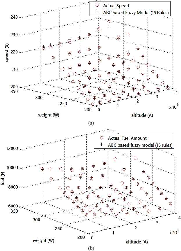
ABC algorithm based fuzzy model results for (a) speed, and (b) fuel variables (CS=30)

DE algorithm based fuzzy model results for (a) speed, and (b) fuel variables (CS=40)

Comparison of the algorithms for (a) speed and (b) fuel test data in 16-rules fuzzy models
Figures 3–4 show fairly good agreement of the model results with the actual values. The representation in Figure 5, which provides a comparison of the algorithms for the test data in 16-rules fuzzy models, confirms this interpretation. The actual values and fuzzy model results for train and test operations are listed in Table 4 in order to better evaluate the performance of the models. Percentage errors between training and test data are shown in Figure 6 and Figure 7.
| Actual Outputs | 16-Rules Fuzzy Model Outputs | Actual Outputs | 16-Rules Fuzzy Model Outputs | ||||||||
|---|---|---|---|---|---|---|---|---|---|---|---|
| ABC based Model (PI=0.0011) | DEA based Model(PI=0.0010) | ABC based Model (PI=0.0011) | DEA based Model (PI=0.0010) | ||||||||
| Speed | Fuel | Speed | Fuel | Speed | Fuel | Speed | Fuel | Speed | Fuel | Speed | Fuel |
| 225 | 10620 | 226.02 | 10578.41 | 226.23 | 10612.61 | 200 | 6820 | 200.78 | 6834.64 | 200.06 | 6814.89 |
| 221 | 10000 | 220.92 | 10039.79 | 221.00 | 10033.57 | 227 | 9700 | 226.93 | 9681.15 | 227.21 | 9655.01 |
| 216 | 9380 | 215.46 | 9387.18 | 215.78 | 9362.85 | 221 | 9060 | 221.60 | 9087.73 | 222.10 | 9068.18 |
| 213 | 9080 | 212.38 | 9075.28 | 212.66 | 9080.22 | 216 | 8440 | 215.93 | 8398.89 | 216.20 | 8429.16 |
| 210 | 8780 | 209.72 | 8723.96 | 210.10 | 8776.55 | 213 | 8140 | 212.67 | 8113.82 | 213.11 | 8106.33 |
| 207 | 8500 | 207.20 | 8409.35 | 207.61 | 8481.94 | 210 | 7820 | 209.88 | 7809.92 | 210.15 | 7796.36 |
| 205 | 8220 | 204.63 | 8184.68 | 205.19 | 8196.02 | 207 | 7520 | 207.23 | 7562.43 | 207.40 | 7487.82 |
| 202 | 7940 | 201.79 | 7995.19 | 202.81 | 7913.56 | 205 | 7220 | 204.54 | 7231.59 | 204.65 | 7200.69 |
| 200 | 7680 | 200.56 | 7743.54 | 200.90 | 7630.85 | 202 | 6920 | 201.52 | 6903.43 | 201.98 | 6924.69 |
| 225 | 10460 | 226.17 | 10439.39 | 225.41 | 10437.61 | 200 | 6640 | 200.24 | 6681.81 | 199.75 | 6696.12 |
| 216 | 9240 | 215.42 | 9223.44 | 215.18 | 9225.18 | 229 | 9700 | 227.69 | 9702.01 | 227.84 | 9728.25 |
| 213 | 8980 | 212.26 | 8917.52 | 212.42 | 8901.20 | 216 | 8400 | 216.64 | 8377.25 | 216.25 | 8434.79 |
| 210 | 8360 | 209.57 | 8572.48 | 209.75 | 8587.46 | 213 | 8080 | 213.27 | 8086.03 | 213.05 | 8100.09 |
| 207 | 8360 | 207.03 | 8266.87 | 207.16 | 8283.49 | 210 | 7760 | 210.37 | 7777.16 | 209.98 | 7779.26 |
| 205 | 8080 | 204.42 | 8018.91 | 204.77 | 8084.80 | 205 | 7160 | 204.93 | 7176.97 | 204.21 | 7175.71 |
| 202 | 7800 | 201.50 | 7806.32 | 202.42 | 7807.00 | 202 | 6860 | 201.87 | 6832.30 | 201.46 | 6889.00 |
| 200 | 7520 | 200.26 | 7559.37 | 200.53 | 7529.38 | 200 | 6580 | 200.53 | 6608.13 | 199.27 | 6610.67 |
| 225 | 10200 | 226.27 | 10174.68 | 226.05 | 10203.69 | 232 | 9920 | 228.80 | 9887.39 | 229.32 | 9924.32 |
| 221 | 9580 | 221.16 | 9621.87 | 220.71 | 9608.84 | 224 | 9180 | 223.41 | 9251.51 | 222.96 | 9227.19 |
| 216 | 8980 | 215.70 | 8965.50 | 215.08 | 9006.74 | 216 | 8500 | 217.39 | 8508.61 | 216.63 | 8525.63 |
| 213 | 8680 | 212.56 | 8674.24 | 212.19 | 8670.74 | 213 | 8200 | 213.89 | 8192.42 | 213.32 | 8177.47 |
| 210 | 8400 | 209.88 | 8349.95 | 209.39 | 8345.88 | 210 | 7880 | 210.82 | 7862.85 | 210.24 | 7841.89 |
| 205 | 7840 | 204.78 | 7800.74 | 204.44 | 7857.90 | 207 | 7560 | 207.90 | 7602.70 | 207.47 | 7518.82 |
| 202 | 7560 | 201.93 | 7565.00 | 201.98 | 7569.56 | 205 | 7220 | 205.20 | 7221.99 | 204.16 | 7203.65 |
| 200 | 7300 | 200.69 | 7332.18 | 200.00 | 7283.30 | 200 | 6580 | 200.62 | 6618.19 | 199.02 | 6613.57 |
| 225 | 9800 | 226.45 | 9950.36 | 225.39 | 9807.34 | 225 | 10106 | 224.89 | 10109.77 | 223.81 | 10092.44 |
| 221 | 9620 | 221.24 | 9380.21 | 221.94 | 9477.41 | 218 | 9100 | 218.02 | 9083.85 | 218.38 | 9104.26 |
| 216 | 8660 | 215.68 | 8712.91 | 215.77 | 8756.86 | 214 | 8600 | 214.16 | 8591.05 | 214.96 | 8582.66 |
| 213 | 8380 | 212.48 | 8427.63 | 212.57 | 8391.49 | 210 | 8160 | 210.65 | 8167.00 | 211.71 | 8168.41 |
| 210 | 8120 | 209.78 | 8109.78 | 209.59 | 8122.79 | 207 | 7820 | 207.77 | 7845.14 | 208.55 | 7800.72 |
| 207 | 7840 | 207.21 | 7842.12 | 206.69 | 7790.32 | 205 | 7500 | 204.90 | 7506.07 | 205.53 | 7481.51 |
| 205 | 7560 | 204.59 | 7548.69 | 204.38 | 7625.57 | 202 | 7200 | 201.61 | 7158.35 | 202.53 | 7173.62 |
| 202 | 7280 | 201.65 | 7277.73 | 201.75 | 7321.94 | 200 | 6860 | 200.19 | 6876.94 | 200.15 | 6881.23 |
| 200 | 7020 | 200.40 | 7054.12 | 199.65 | 7022.82 | 221* | 9840* | 220.94 | 9889.21 | 220.69 | 9833.88 |
| 226 | 9680 | 226.25 | 9678.88 | 226.48 | 9666.53 | 207* | 8100* | 207.34 | 8066.25 | 206.69 | 8031.61 |
| 221 | 9060 | 221.21 | 9109.66 | 221.32 | 9094.82 | 213* | 8200* | 212.62 | 8189.39 | 212.84 | 8136.87 |
| 216 | 8480 | 215.76 | 8457.86 | 215.76 | 8465.74 | 205* | 7360* | 204.86 | 7341.74 | 204.71 | 7324.76 |
| 210 | 7920 | 209.96 | 7893.78 | 210.55 | 7961.10 | 221* | 9020* | 222.41 | 9047.95 | 222.39 | 9114.16 |
| 207 | 7640 | 207.41 | 7649.12 | 207.62 | 7630.28 | 207* | 7460* | 207.64 | 7520.71 | 207.04 | 7471.39 |
| 202 | 7080 | 202.02 | 7052.03 | 201.95 | 7013.40 | 202* | 6880* | 202.03 | 6855.07 | 201.25 | 6897.74 |
Test Data
Actual values and the outputs of 16-rules fuzzy models for speed and fuel variables
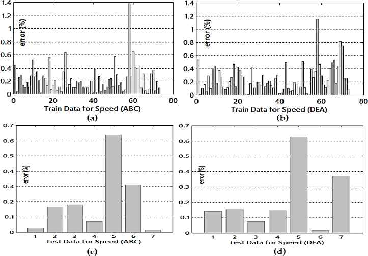
Percentage errors in speed parameter (a) for train data by ABC (b) for train data by DEA (c) for test data by ABC (d) for test data by DEA
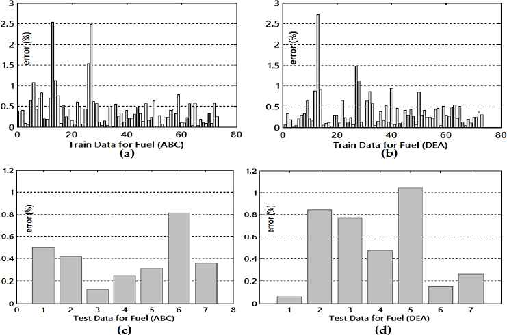
Percentage errors in fuel parameter (a) for train data by ABC (b) for train data by DEA (c) for test data by ABC (d) for test data by DEA
In our other study presented in Ref.[7], which includes simultaneous calculation of speed and fuel, the results of the Anfis and neural network models are presented. In that study based on the MSE value, when the training and test data were evaluated together, it was stated that the generalized regression neural network (GRNN) approach comes to the forefront. In this model, the MSE values are obtained as follows: MSE(train)=0.06 and MSE(test)=0.3 for speed; MSE(train)=898.46 and MSE(test)=2888.19 for fuel7.
Furthermore, in the 16-Rules Anfis model given in Ref.[7], which uses triangular type membership functions, the following values are reached: MSE(train)=0.09 and MSE(test)=0.44 for speed; MSE(train)=2173.03 and MSE(test)=1589.27 for fuel. On the other hand, for the DE algorithm based fuzzy model which gives the best PI value in our study, these values are noted in Table 3 as follows: MSE(train)=0.4868 and MSE(test)=0.3991 for speed; MSE(train)=1992 and MSE(test)=2750.3 for fuel. Numerous studies in the literature have shown that each of these artificial intelligence based approaches has different specific properties and application advantages. Nevertheless, these values can provide a general idea for a rough comparison. In any case, the results obtained in this study clearly indicate once again that a quite impressive and competitive performance can be achieved using the fuzzy logic -based modeling approach.
From Figure 6 and Figure 7, it is possible to say that the performances of both algorithms are close to each other. In the training process, while the maximum percentage error values obtained for models based on the ABC and DE algorithms for the speed parameter are 1.38 and 1.16, these values for the fuel parameter are 2.54 and 2.72, respectively. In the test process, the ABC and DE based fuzzy models cause the maximum percentage error values of 0.64 and 0.63 for the speed parameter, 0.81 and 1.04 for the fuel parameter, respectively. These results can be evaluated as quite satisfactory and show the ability of both algorithms to successfully obtain the fuzzy model parameters.
The variation of the PI error value according to the iterations in the 16-rules fuzzy modeling process is comparatively presented in Figure 8 for both algorithms. From the variation given for the first 2000 iterations, it is seen that the DE algorithm reduces the error value at lower iterations than the ABC approach. Undoubtedly in this case, better solutions can be achieved in shorter time. According to the figure, in order for the ABC algorithm to provide the PI value achieved by the DE algorithm, a 1000 iteration time has to pass. This is important in that the DE algorithm has the advantage of rapid convergence.
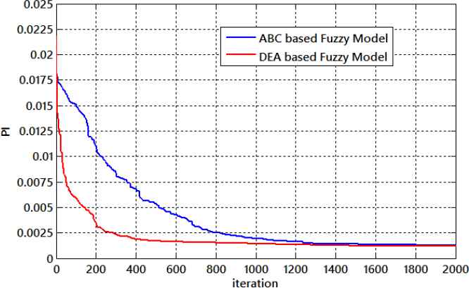
Iteration-PI variation for ABC and DE based fuzzy models with 16 rules
The most important feature that distinguishes this work from our fuzzy logic based other studies is the simultaneous determination of more than one output. From the results obtained, it is seen that high model success cannot be achieved by the low number of rules. The main reason for this is that two outputs with high nonlinearity are tried to be provided with the minimum error at the same time. To overcome this difficulty, in this study, a performance index defined as PI is used to determine the fuzzy rule parameters. Thus, as expected, a good model performance that can be considered successful when the number of rules increases is achieved. And, it is possible to provide simultaneously multiple outputs compatible with the measurement results. Furthermore, it can also be said that the performance of the fuzzy model can be significantly improved when the fuzzy model parameters are obtained by ABC or DE algorithm.
5. Conclusions
In order to maximize the safety of life and property, the information obtained from the sensors at many points of the aircrafts must be accurately, precisely and quickly evaluated by the flight control system and decision support mechanisms. Admittedly, the use of a model that accurately interprets complex measurement data provides great support to pilots in making the required decisions at critical moments. In this study, a fuzzy modeling study is carried out using a complex data set of an exemplary flight control system. For this purpose, speed and fuel output values were tried to be obtained simultaneously according to altitude, weight, engine pressure ratio input information of Boeing B-767-200ER type aircraft. Fuzzy model parameters including different rule numbers are determined using ABC and DE algorithms and presented in a comparative form. From this study, which provides important findings to show the power of the fuzzy model structure presented and the heuristic algorithms used, it is seen that the actual and fuzzy model outputs are very compatible with each other and that the algorithms provide remarkable success in finding fuzzy model parameters with double output.
Acknowledgements
This work was supported by Research Fund of the Erciyes University. Project Number: FDK-2014-5032.
References
Cite this article
TY  - JOUR
AU  - Aytekin Bagis
AU  - Mehmet Konar
PY  - 2018
DA  - 2018/02/09
TI  - ABC and DE Algorithms based Fuzzy Modeling of Flight Data for Speed and Fuel Computation
JO  - International Journal of Computational Intelligence Systems
SP  - 790
EP  - 802
VL  - 11
IS  - 1
SN  - 1875-6883
UR  - https://doi.org/10.2991/ijcis.11.1.60
DO  - 10.2991/ijcis.11.1.60
ID  - Bagis2018
ER  -