
Reduction of carbon emission and total late work criterion in job shop scheduling by applying a multi-objective imperialist competitive algorithm
- DOI
- 10.2991/ijcis.11.1.62How to use a DOI?
- Keywords
- Job shop scheduling; environmentally sustainable operations management; carbon footprint; late work criterion; multi-objective imperialist competitive algorithm; multi-objective optimization problem
- Abstract
New environmental regulations have driven companies to adopt low-carbon manufacturing. This research is aimed at considering carbon dioxide in the operational decision level where limited studies can be found, especially in the scheduling area. In particular, the purpose of this research is to simultaneously minimize carbon emission and total late work criterion as sustainability-based and classical-based objective functions, respectively, in the multi-objective job shop scheduling environment. In order to solve the presented problem more effectively, a new multi-objective imperialist competitive algorithm imitating the behavior of imperialistic competition is proposed to obtain a set of non-dominated schedules. In this work, a three-fold scientific contribution can be observed in the problem and solution method, that are: (1) integrating carbon dioxide into the operational decision level of job shop scheduling, (2) considering total late work criterion in multi-objective job shop scheduling, and (3) proposing a new multi-objective imperialist competitive algorithm for solving the extended multi-objective optimization problem. The elements of the proposed algorithm are elucidated and forty three small and large sized extended benchmarked data sets are solved by the algorithm. Numerical results are compared with two well-known and most representative metaheuristic approaches, which are multi-objective particle swarm optimization and non-dominated sorting genetic algorithm II, in order to evaluate the performance of the proposed algorithm. The obtained results reveal the effectiveness and efficiency of the proposed multi-objective imperialist competitive algorithm in finding high quality non-dominated schedules as compared to the other metaheuristic approaches.
- Copyright
- © 2018, the Authors. Published by Atlantis Press.
- Open Access
- This is an open access article under the CC BY-NC license (http://creativecommons.org/licences/by-nc/4.0/).
1. Introduction
In the last decades, various reports on environmental issues have been released, in which they are stating the escalating deterioration of the environment that is mainly caused by the world population activities. In a report issued by Stocker et al.1, it is stated that the amount of greenhouse gases has markedly increased in the atmosphere, including carbon dioxide, nitrous oxide, methane, etc. Among these greenhouse gases, carbon dioxide is the major contributor to global warming, and it is mainly emitted from industrial processes, power plants, transportation activities, etc. In particular, electricity generation from fossil fuels accounts for a significant portion of carbon dioxide emission. Although the average carbon dioxide intensity has declined by 3% over the years from 1980 to 2010, its emission rate has increased by a factor of 72% over the same period.2 For example, in the U.S., 82 % of the total emitted greenhouse gases is carbon dioxide.3 Moreover, the industrial sector in the U.S. accounts for 27.5% of carbon dioxide with the highest annual growth rate projection (0.5%) in comparison with other sectors.4
From the production management viewpoint, reducing carbon emission can be tackled from three levels including strategic, tactical, and operational that are based on time horizon.5 In the strategic level, carbon emission can be considered for long-lasting decisions with higher investments such as supply chain network design in locating plants and warehouses.6, 7 In the tactical level, carbon dioxide can be integrated in decisions regarding production and distribution such as inventory and lot sizing models.8, 9 In the operational level, carbon dioxide can be integrated in scheduling problems such as batch scheduling and hybrid flow shop scheduling problems.10
Previously, research attempts in manufacturing scheduling have mainly focused on reducing makespan, buffer size, tardiness, mean flow time, etc.11–13, while neglecting eco-efficient-based objective functions. To date, as a research gap, eco-efficient-based objective functions have not been considered in the job shop scheduling environment.10, 14, 15 The job shop manufacturing system is important because many real-world enterprises are adopting it. This paper will thus address the following research questions: (1) How an eco-efficient-based objective function and a classical-based objective function can be simultaneously minimized in the job shop scheduling environment? (2) How this multi-objective job shop scheduling problem can be solved? Due to the scarcity of research done on carbon footprint reduction in the operational decision level, the main motivation of this paper is to model a green multi-objective job shop scheduling problem that is aimed at optimizing two objectives, simultaneously. Specifically, it reduces carbon footprint as the green or eco-efficient objective. At the same time, it minimizes the total late work criterion as the classical objective, which is an aspect neglected by previous studies. Based on the fact that the scheduling objectives are usually in conflict with each other, a new multi-objective imperialist competitive algorithm (MOICA) is proposed to generate a set of non-dominated solutions for the presented problem. This is the first attempt at solving job shop scheduling problems with carbon footprint and total late work criterion objective functions by applying MOICA, i.e. a three-fold scientific contribution. To demonstrate the performance of the proposed MOICA, a set of extended benchmarked data sets is used. In addition, the numerical results are compared with two famous and common multi-objective algorithms16, which are non-dominated sorting genetic algorithm II (NSGA-II) and multi-objective particle swarm optimization (MOPSO). This is conducted to reveal the effectiveness and efficiency of the proposed MOICA.
The remaining contents of this paper are organized as follows. Literature review and research gaps are presented in section 2. In section 3, the multi-objective job shop scheduling problem with carbon emission and total late work criterion is described, and its mathematical model is constructed. In section 4, the proposed MOICA is presented. Computational experiments and discussions are provided in section 5. Finally, conclusions and future research opportunities are given in section 6.
2. Literature Review
According to Zhang and Wang17, solely considering technology innovation cannot be an efficient approach for reducing carbon emission. Operational decisions and policies including business practices are significant factors and drivers for reducing carbon emission than considering physical processes.18 On one hand, published studies on carbon emission reduction in manufacturing have mainly focused on designing and developing new machineries and equipment.19–22 On the other hand, previous research has also considered reducing carbon emission through product design and operational decisions.23–25 Albeit the machine-level and product-level viewpoints can support carbon reduction, both perspectives require a considerable amount of financial investments.
This research, unlike machine-level and product-level studies, attempts to minimize carbon emission in the operational decision level from the manufacturing system perspective. Limited research can be found in this area, especially in the job shop scheduling environment. Zheng and Wang15 presented a multi-objective project scheduling problem that aims at minimizing carbon emission and makespan. In addition, they proposed a Pareto-based estimation of distribution algorithm to obtain a set of Pareto solutions in order to balance benign manufacturing criterion and production effectiveness. Liu14 investigated a multi-objective batch scheduling problem to minimize carbon emission and total weighted tardiness, and presented an ε-archived genetic algorithm to solve it. Liu and Huang10 addressed a batch scheduling and hybrid flow shop problem to minimize carbon footprint, energy consumption, and total weighted tardiness by applying a non-dominated sorting genetic algorithm. For a recent and comprehensive survey on multi-objective production scheduling, interested readers can refer to Lei.26 It should be noted that carbon footprint reduction in the industrial sector can be recognized as one of the top future research challenges, especially from the operations research perspective. Based on the reviewed studies, limited research can be seen in low-carbon scheduling, and no research attempt has been made in low-carbon job shop scheduling problems.
Due date related performance measures such as total tardiness, total late work criterion, and total lateness are useful criteria in scheduling. The total late work criterion is a special case of total tardiness which was first proposed by Blazewicz.27 This criterion is a performance measure that accounts for the late part of each operation, in which it is calculated by summing the durations of late parts of all operations. The total late work criterion can be considered significant from the manufacturers’ and customers’ perspectives. On one hand, manufacturers aim at delivering products on time or before their due dates to maximize profits by minimizing the agreed penalties upon the late parts of each order. On the other hand, customers aim at receiving products on time or with least late parts of each order. Therefore, the total late work criterion is minimized to account for the minimum late parts of each customer’s order. This criterion has been applied on single machine scheduling28, 29, resource constrained project scheduling30, identical parallel processors scheduling31, flow shop scheduling32–35, open shop scheduling36, and flexible manufacturing scheduling.37 Interested readers on the late work criterion can refer to a state-of-the-art literature survey performed by Sterna.38 However, to the authors’ best knowledge, except for a theoretical study39, there is no research in job shop scheduling that considers the late work criterion, especially in the multi-objective area.
A multi-objective job shop scheduling problem is complex and non-deterministic polynomial-time hard (NP-hard) and it cannot be solved by exact methods. Hence, metaheuristic approaches are the most appropriate methods to solve it. Metaheuristics imitate social behaviors, physical processes, imperialistic competitions, nature, etc. Many of them have been adopted in production scheduling, specifically in job shop scheduling problems, such as genetic algorithm11, 40, 41, memetic algorithm42, water drops algorithm13, variable neighborhood search43, immune algorithm44, 45, evolutionary algorithm46, 47, and particle swarm optimization.48–50 Among the metaheuristic approaches, the imperialist competitive algorithm (ICA) is a population-based algorithm that was presented by Atashpaz-Gargari and Lucas51 So far, the ICA-based approaches have been applied on different multi-objective optimization problems that were aimed at providing a set of Pareto optimal solutions, such as assembly line design 52, coupling of photovoltaicelectrolyzer system53, sensor deployment in wireless sensor networks54, and benchmarked functions.55, 56 Hosseini and Al Khaled57 have presented a state-of-the-art literature survey on the application of ICA in different engineering disciplines. In accordance with the reviewed studies, MOICA has been found to be more efficient than the other approaches for solving engineering problems of different domains. Interestingly, MOICA has not been utilized for solving production scheduling problems, especially multi-objective job shop scheduling problems.
Based on the literature review carried out on the main notions of low-carbon production scheduling, total late work criterion, and multi-objective metaheuristic approaches, the following gaps can be observed. (1) Previously, research attention has mainly concentrated on minimizing classical-based objective functions such as makespan, lateness, tardiness, etc., while ignoring eco-efficient-based objective functions, especially in job shop scheduling. (2) In addition, previous researchers have not considered the total late work criterion, as a classical-based objective function, in multi-objective job shop scheduling. (3) Moreover, ICA as a newly developed and efficient metaheuristic approach has not been applied on multi-objective scheduling problems, especially low-carbon multi-objective job shop scheduling problems. Therefore, this research aims to fill these gaps by developing a multi-objective mixed-integer mathematical model with the objectives of simultaneously minimizing carbon footprint and total late work criterion, as eco-efficient-based and classical-based objective functions, respectively, in the job shop scheduling environment. This research also proposes a new MOICA in order to solve the problem and obtain a set of non-dominated solutions for the conflicting objectives.
3. Problem Description and Multi-objective Model Formulation
3.1. Problem description and characteristics
In a job shop environment, jobs are independent of each other with different routes where machines are organized based on processes; that is, machines are grouped in work-centers with similar processing capabilities. In addition, parts are transferred across different work-centers according to their process plan where machines are capable of processing a large variety of parts. In a job shop scheduling problem, a set of n jobs J = {Jj=1, J2, J3,…, Jn} is to be executed on a set of m machines M = {Mi=1, M2, M3,…, Mm} according to the technological sequences. Each job has a set of l ordered operations O = {O1j, O2j, O3j,…, Olj} where Olj is the lth operation of job j assigned to a prior known machine with a known processing time. The start time of Olj on its specified machine will be decided based on the production schedule. The goal is to sequence all operations of jobs on all machines while minimizing or maximizing certain objective functions.
The following assumptions and characteristics are considered for the problem under study, as unique conditions impose different problems in scheduling. (1) An operation of a job cannot be executed by more than one machine at the same time and a machine cannot process more than one operation simultaneously in order to avoid overlapping in operations and machines, respectively. (2) Operations of a job are nonpreemptable; that is, once an operation is commenced on a machine, its temporary interruption is not permitted. (3) Recirculation of operations (twice-visiting a machine) is not considered. (4) Emitted carbon dioxide per kilowatt hour of consumed energy is a constant. (5) Buffer size between machines is unlimited. (6) Setup time, as well as loading and unloading time are assumed to be negligible, or are included in an operation’s processing time. (7) Machines and jobs are constantly available from time zero. (8) There is no interdependency among operations of different jobs.
3.2. Proposed multi-objective mathematical formulation
The indexes, parameters, variables, and mathematical model for the problem described above with the objectives of minimizing the total late work criterion and carbon dioxide simultaneously are given below.
Index of machines Index of jobs Index of idle states Index of operations Index of priorities Number of machines Number of jobs Number of idle states of a machine Number of operations lth operation of job j Processing time of Olj on machine i Due date of job j Power consumption of machine i in processing condition Power consumption of machine i in idle condition Quantity of emitted carbon dioxide per kilowatt hour It is assumed as a big number Completion time of Olj on machine i Start time of Olj on machine i Start time of ith machine in the pth priority Duration of kth idle state for machine i Total late work criterion of the schedule Total emitted carbon footprint of the schedule
Mathematical model
Equations (1) and (2) account for the first and second objective functions to minimize the total late work criterion (TLWC) and total emitted carbon footprint (TLWC), respectively. In order to calculate the late work criterion for an operation, firstly, the due date of job j should be subtracted from the completion time of lth operation of job j executed on machine i
4. Multi-objective Imperialist Competitive Algorithm (MOICA) for the Job Shop Scheduling Problem
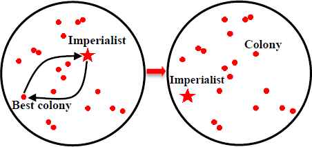
As mentioned earlier, a new MOICA is proposed to solve the presented low-carbon multi-objective job shop scheduling problem. ICA is a recently developed evolutionary approach51 which imitates imperialistic competitions and socio-political behaviors. Particularly, developed countries are inclined to compete vigorously for capturing weak and undeveloped nations to gain dominance over their natural resources and political issues. The imperialists aim to advance their politics, economy, and military, and to spread their own cultural values and norms in the colonial countries. This imperialistic competition brings down and collapses the weakest empires but strengthens the powerful empires.
In the proposed MOICA, the following operators are new or modified based on the problem’s characteristics: (1) A modified encoding and decoding of solutions. (2) A modified imperialistic selection and colonial distribution. (3) Information sharing by using crossover operators, namely, uniform crossover, one-point crossover, two-point crossover, and precedence preserving order-based crossover. (4) Revolution operators, namely, swap, insert, inverse, and perturbation. (5) Inter-empire competition by applying the roulette wheel selection technique. The following sections provide a stepwise delineation of the proposed MOICA.
4.1. Encoding and decoding of solutions
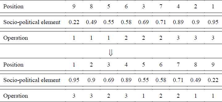
In a metaheuristic algorithm, encoding and decoding of a solution is an important decision. In the proposed MOICA, a solution consists of Nvar variables and it is represented by a matrix. A country is defined as [pi=1, p2,…,pNvar] where pi is the value of the ith variable which stands for a socio-political element, such as religion, language, economy, culture, race, etc. The algorithm searches for the best combination of these socio-political variables in each country to generate a set of Pareto-optimal countries. In addition, an operation-based representation is adopted to encode the solution of the job shop scheduling problem.58 In this representation scheme, integer variables starting from 1 to n, where n denotes the number of jobs, indicate the sequencing of operations that should be performed on the machines. In addition, each integer variable should be repeated s times within the length of a solution matrix, where s denotes the number of operations of a job. In Fig. 1, an encoding scheme of a small job shop scheduling instance with 3 jobs, 3 operations for each job, and 3 machines is presented. In this figure, the first row shows the position of each socio-political variable, the second row shows the socio-political variable values of a country which are represented by floating point numbers, and the third row shows the sequencing of operations for each job. In order to assign the operations, firstly, the socio-political variables are sorted in ascending order; secondly, the operations of jobs starting from 1 to n are assigned from the most left to the most right. Thirdly, the socio-political variables and assigned operations are sorted based on their recorded positions (values in the first row). It should be noted that each country is composed of additional information, including processing time, machine number, power consumption, etc. that are attached to it.
Encoding scheme of a job shop scheduling problem for the proposed MOICA
In order to decode the solution and construct a feasible schedule, the first element of the operations in the most left side should be scheduled first, continued by the second element, until the last element of the operations. In Fig. 1, for instance, the first operation of job 3, second operation of job 3, first operation of job 2, third operation of job 3, first operation of job 1, second operation of job 2, third operation of job 2, second operation of job 1, and third operation of job 1 should be scheduled one after another by considering the process and time constraints, respectively. The adopted procedures for encoding and decoding the solutions can guarantee the feasibility of the generated schedules.
4.2. Initialization and generation of empires
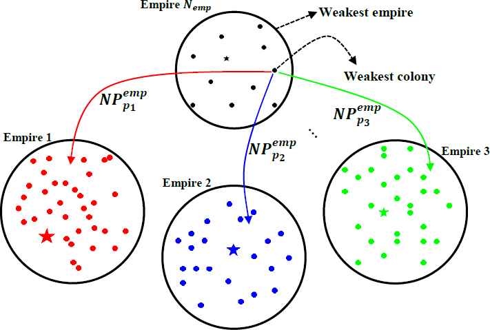
In the proposed algorithm, the best combination of socio-political variables such as language, race, and economic policy is desired in order to form a country with minimum objective function values. To initialize and begin the algorithm, a population of size Npop is randomly generated by sampling from all the feasible solutions. Then, initial countries are ranked by a non-dominated technique in order to extract and form different Pareto front solutions.59, 60 In addition, each country is assigned a value called crowding-distance to keep each front as diverse as possible.59 In the next step, countries are sorted based on their crowding-distance in descending order; then, they are sorted based on their rank in ascending order. In other words, countries with a lower rank and higher crowding-distance are powerful. The powerful countries in terms of rank and crowding-distance are selected with the size of Nimp as the imperialists. The remaining countries, however, are considered as colonial countries with the size of NCol, in which they should be distributed among the empires based on the imperialists’ power (see Fig. 2). To compute the power of each imperialist, firstly, the normalized cost of the ith objective function for imperialist n, denoted by NCi,n, should be computed according to Eq. 15,
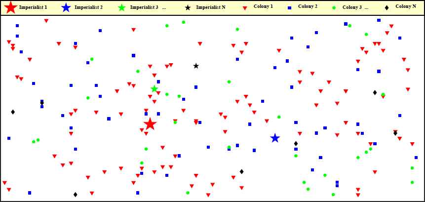
Initializing imperialists and colonies to form the initial empires
4.3. Total power of an empire
The total power of an empire is computed based on the total normalized cost of its imperialist and the total normalized cost of its colonies. The total power of an empire, however, is greatly affected by its imperialist and slightly affected by its colonial countries. In Eq. 18, the total power of the kth empire, denoted by
4.4. Moving the colonies of an empire towards its imperialist (Assimilation)
In each empire, an imperialistic country attempts to improve its colonies by assimilating and changing their socio-political variables, such as changing their languages, building new schools, changing their religions, improving their cultures, etc. This fact is simulated by an operator called assimilation in order to move the colonies of an empire towards the imperialistic country by x units in the direction of θ. The original position of a colony is moved x units towards its imperialist, in which x is randomly sampled from a uniform distribution as follows,
In addition, a random deviation of θ is added to the movement direction of colonies to discover new positions of colonies around the imperialist, in which θ is randomly sampled from a uniform distribution as follows,
4.5. Information sharing by crossover
In each empire, colonial countries can enhance and improve their socio-political elements by information sharing with each other, in which it can be performed by adopting a crossover operator. In information sharing, colonies selection is carried out by applying the tournament selection technique, where the best colonies in terms of rank and crowding-distance will have higher chances of selection than the others. In the tournament selection technique, firstly, a set of colonies is randomly selected based on an arbitrary tournament size of 5. Secondly, if the randomly selected colonies are from different fronts, the lowest ranked colony is selected among them as the best colonial country for information sharing. Otherwise, if the randomly selected colonies are from the same front, the lowest ranked colony with the highest crowding-distance is selected among them as the best colonial country for information sharing. In this paper, four different types of crossover operators, including precedence preserving order-based crossover, one-point crossover, two-point crossover, and uniform crossover are applied for information sharing between the colonial states. As shown in Figs. 3 and 4, one-point crossover, two-point crossover, and uniform crossover are applied on the continuous part of the colonies, while precedence preserving order-based crossover is applied on the discrete part of the colonies, i.e. sequencing part. In addition, in each iteration of the empires, one of these operators is randomly selected for information sharing between the colonial states.
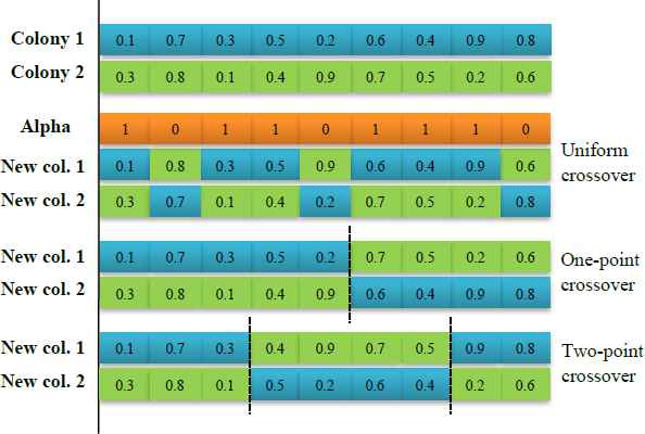
Information sharing between colonies of an empire by applying crossover operators on the continuous part of the solutions

Information sharing between colonies of an empire by applying a crossover operator on the discrete part of the solutions
4.6. Revolution
Colonial countries are usually dominated by their relevant imperialist in terms of socio-political variables; however, some colonial states might not be dominated or absorbed by their imperialist. These colonial states might revolt to improve their socio-political variables, where this fact is simulated in the proposed MOICA by adopting a revolution operator. This operator increases exploration, while decreases the risk of getting trapped in local optima. In each iteration of the empires, the revolution operator is performed on a percentage of randomly selected colonies. In order to revolutionize some colonial states, different operators are designed, including swap, insert, and inverse operators, where these operators are applied on the discrete part of the solutions as shown in Fig. 5. Besides applying them, a perturbation operator is applied on the continuous part of the colonial states. In the perturbation operator, two socio-political variable values are randomly selected and replaced with two randomly generated socio-political variable values. It is noted that one of the aforementioned operators, including perturbation, swap, insert, and inverse is randomly selected to revolutionize the continuous or discrete part of the colonial states.
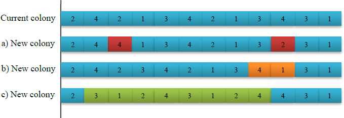
An example of revolution operators: a) swap, b) insert, and c) inverse
4.7. Updating colonial states of an empire
In each iteration of the empires, obtained or generated colonial states by assimilation, information sharing, and revolution, and initial colonial states are merged together to form the potential colonies, in terms of improved socio-political variables, for the corresponding empire. In this step, firstly, colonial states with the same objective function values are removed from the merged population in order to prevent duplication of colonies. In the next phase, merged colonies are sorted based on crowding-distance and rank in descending and ascending order, respectively. Then, better colonial states in terms of rank and crowding-distance are selected with the size of
4.8. Intra-empire competition
While performing assimilation, information sharing, and revolution within an empire, a colonial state may reach a position with a lower total normalized cost than its imperialist. Intra-empire competition happens inside an empire between the colonial states and imperialist to exchange the position of the imperialist with the best colonial state. After exchanging the positions, colonial states move towards the new position of the imperialist; that is, the rules of the imperialist and colonial state change accordingly. The exchange of positions for an imperialist and the best colonial state are presented in Fig. 6.
Intra-empire competition between the best colonial state and imperialist
4.9. Inter-empire competition
Imperialistic countries compete with each other to seize the weak and undeveloped colonial states in order to increase their own power. As depicted in Fig. 7, inter-empire competition happens among the empires for possessing the weakest colonial state of the weakest empire, where the power of a powerful empire increases and the power of a feeble empire decreases. In the inter-empire competition, albeit, the most powerful empire is the most possible winner for seizing the weakest colony of the weakest empire, it is not a certain winner, and each empire has a likely chance of winning. To begin the inter-empire competition, firstly, the weakest colonial state of the weakest empire is selected. Then, the possession probability of each empire is calculated according to Eq. 21,
Inter-empire competition for possessing the weakest colony of the weakest empire
Moreover, in the inter-empire competition, a feeble empire without any colonial state will collapse and its imperialist will be given as a colonial state to the winning empire (see Fig. 8). It is noted that a collapsed empire wil l be removed from the empires. The flowchart of the proposed MOICA is depicted in Fig. 9.

Collapsing a feeble empire without any colonial state
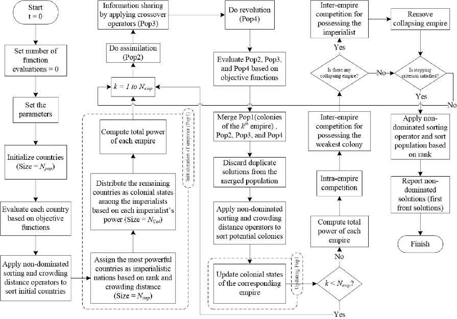
Flowchart of the proposed MOICA
4.10. Stopping condition
In the proposed MOICA, a single condition is provided to terminate the algorithm, where the number of function evaluations is set as the terminating condition.
5. Computational experiments
The explicit aim of this section is to validate the effectiveness and efficiency of the proposed MOICA by comparing it with two well-known and common multi-objective metaheuristic approaches which are NSGA-II and MOPSO.59,62 They were selected for comparison because they have been employed by many researchers in the recent years to evaluate and validate the effectiveness of their own multi-objective metaheuristic approaches. In this paper, NSGA-II and MOPSO adopted the same solution encoding and decoding as the proposed MOICA. The procedures or steps of NSGA-II and MOPSO followed those presented by Deb et al.59 and Coello et al.62, respectively. All the three multi-objective metaheuristic approaches were coded in MATLAB programming language R2010a, and they were tested on a personal computer with Intel(R) Core(TM) Duo CPU T2450 at 2.00 GHz, and 2.5 GB of main memory.
5.1. Extended benchmarked data sets
To systematically evaluate and validate the performance of the proposed MOICA, a set of 43 well-studied and common benchmarked instances was collected from the Operations Research library website at the Brunel University London.63 The considered benchmarked instances are exhaustive, in terms of machines, jobs, size of problems (i.e. from small to large), and level of difficulties, which are prefixed by LA01-LA40, FT06, FT10, and FT20. In addition, these basic benchmarked problems contain the jobs, operations of each job, machines, and technological sequencing of each job. Based on the fact that the investigated green multi-objective job shop scheduling problem is a newly extended problem in some aspects, the considered benchmarked data sets are extended to include all the other required information, including the power consumption in processing condition, power consumption in idle duration, quantity of emitted carbon dioxide, and due dates. The required information is generated and elucidated as follows.
- •
A machine’s power consumption in processing state is randomly generated from a uniform distribution U(5,18).
- •
A machine’s power consumption in idle state is randomly produced from a uniform distribution U (1,3) The generated power consumption data in processing state and idle state are tabulated and presented in Appendices A and B, respectively.
- •
Emitted carbon dioxide from electricity generation by using coal, natural gas, and other fossil fuels is a constant, and it is assumed to be equal to 0.76 kg Co2 per kilowatt hour.64
- •
In Eq. 23, dj is the due date of the jth job, rj is the release time of the jth job, c = 1.2, 1.5, and 2 is the tightness factor, and
5.2. Performance criteria for algorithms evaluation
It is difficult to make a comparison of the different multi-objective metaheuristics by adopting a single comparison metric, for instance objective function, for performance evaluation in order to validate the effectiveness and efficiency of the proposed MOICA. The following performance criteria, namely, quality metric, mean ideal distance, diversification metric, spacing metric, and number of non-dominated solutions are used for performance evaluation.
- •
Quality Metric (QM): To compute the QM of each algorithm, firstly, all the non-dominated solutions that are obtained by MOICA, MOPSO, and NSGA-II are merged together, and then the non-dominated solutions of the merged solutions are obtained. Subsequently, the share of each algorithm from the extracted non-dominated solutions is calculated in percentage. It is noted that a higher value of this metric is desired.
- •
Mean Ideal Distance (MID): This comparison metric measures the closeness of the ideal points and non-dominated solutions according to each objective function value. In order to compute the MID, Eq. 24 is used, where f1i and f2i are the first and second objective function values of the ith nondominated solution,
- •
Diversification Metric (DM): This comparison metric measures the spread of the non-dominated solutions set for each algorithm according to Eq. 25, where a higher value of this metric is desired.
- •
Spacing Metric (SM): It computes the uniformity of the spread of the non-dominated solutions set according to Eq. 26,
where - •
Number of Non-Dominated Solutions (NNDS): It reports the total number of non-dominated solutions achieved by the algorithm, where a higher value of this metric is desired.
5.3. Parameter setting
The search behavior and performance of the developed MOICA can be significantly affected by a number of parameters, including the population size of countries, Npop, number of imperialists, Nimp, assimilation coefficient, β, probability of information sharing for the population, Pinf, probability of revolution for the population, Prev, and mean total normalized cost of colonies’ coefficient, ξ. After testing with different combinations of the parameters, two levels were chosen for each parameter in order to determine the best combination of the parameters in the proposed MOICA. Therefore, 26 (i.e. 64) situations existed for each randomly selected test instance. Specifically, three test instances with different sizes (LA16, LA29, and LA38) were randomly selected for tuning the proposed approach. Subsequently, all the situations were tested for each of the selected instances and the proposed MOICA was examined according to these settings. The comparison metrics, including QM, MID, DM, SM, and NNDS, were employed in each experiment as performance criteria in which their importance weights were three, two, one, one, and one, respectively. Finally, the best parametric values of the proposed MOICA are tabulated in Table 1. In MOPSO, the significant parameters were the number of particles, Npop, size of the repository, Repsize, number of divisions, Ndiv and mutation rate for a selected particle, µ. After testing with different settings, two levels were chosen for each parameter to determine the best combination of the parameters, where 24 (i.e. 16) situations existed for each of the randomly selected benchmarked problems. Subsequently, all the situations were tested for the selected benchmarked problems and finally, the best combination of the parameters for MOPSO is presented in Table 1. The same approach was employed for tuning the parametric values of NSGA-II. The significant parameters of NSGA-II were the population size, Npop, crossover probability for the population, Pc, mutation probability for the population, Pmu, and mutation rate for a chosen chromosome, µ. The best parametric values of NSGA-II are tabulated in Table 1. It is noted that the number of function evaluations (stopping condition) was set to 80,000 and 130,000 for the small and big sized test instances, respectively, in the proposed MOICA. In addition, the execution time of each problem was recorded for MOICA, and the other metaheuristics were run with the same execution time to ensure a fair comparison.
| MOICA | MOPSO | NSGA-II |
|---|---|---|
| Npop = 100 | Npop = 100 | Npop = 100 |
| Nimp = 10 | Repsize = 100 | Pc = 0.7 |
| β = 2 | Ndiv = 30 | Pmu = 0.4 |
| Pinf = 0.8 | μ = 0.1 | μ = 0.02 |
| Prev = 0.3 | ||
| ξ = 0.1 |
Parameter settings of MOICA, MOPSO, and NSGA-II
5.4. Computational results
In this section, the performance of the proposed MOICA is evaluated in comparison with MOPSO and NSGA-II. The results of the comparison metrics, including QM, MID, DM, SM, and NNDS, are reported in average of five independent runs for each benchmarked instance.
The obtained results are tabulated in Table 2 for the 43 test problems. In this table, the first and second columns show the instance name and instance size while the remaining columns present the values of QM, MID, DM, SM, and NNDS for MOICA, MOPSO, and NSGA-II, respectively. According to these metrics, the optimal solutions obtained by MOICA are generally better than those of the other algorithms. For instance, the obtained non-dominated solutions of LA39 reveal that MOICA is the best one with respect to the first comparison metric, QM = 1, while the share of the other algorithms for this metric equals to 0 (a higher value of QM is desired). The results also show that MOICA is the best approach according to the second comparison metric, MID = 254.786, while the other approaches have higher values for this metric (a lower value of MID is desired). According to the third comparison metric, MOICA is the best algorithm, with DM = 348.226, while the other algorithms have lower values (a higher value of DM is desired). Another comparison metric, SM = 0.662, shows that MOICA is moderately good (a lower value of SM is desired). Finally, MOICA is the best algorithm in achieving a higher number of non-dominated solutions, NNDS = 21 (a higher value of NNDS is desired). The results of other test problems can be interpreted in the same manner.
| Instance Name | Size | QM |
MID |
DM |
SM |
NNDS |
||||||||||
|---|---|---|---|---|---|---|---|---|---|---|---|---|---|---|---|---|
| MOICA | MOPSO | NSGA-II | MOICA | MOPSO | NSGA-II | MOICA | MOPSO | NSGA-II | MOICA | MOPSO | NSGA-II | MOICA | MOPSO | NSGA-II | ||
| FT 06 | 6×6 | 0.400 | 0.267 | 0.333 | 3.679 | 4.602 | 3.624 | 6.073 | 6.662 | 6.074 | 0.445 | 0.173 | 0.407 | 7 | 5 | 7 |
| FT 10 | 10×10 | 0.773 | 0.000 | 0.224 | 328.350 | 675.875 | 363.885 | 516.593 | 321.817 | 384.372 | 0.707 | 0.608 | 0.761 | 21 | 7 | 10 |
| FT 20 | 20×5 | 1.000 | 0.000 | 0.000 | 40.274 | 130.671 | 56.424 | 87.133 | 45.972 | 47.673 | 0.369 | 0.208 | 0.507 | 9 | 3 | 4 |
| LA 01 | 10×5 | 0.640 | 0.000 | 0.360 | 87.850 | 187.73 9 | 112.529 | 212.579 | 216.928 | 260.502 | 0.578 | 0.638 | 0.580 | 16 | 7 | 13 |
| LA 02 | 10×5 | 0.333 | 0.333 | 0.333 | 13.098 | 48.561 | 318.992 | 23.221 | 27.204 | 66.159 | 0.000 | 0.763 | 0.613 | 2 | 3 | 8 |
| LA 03 | 10×5 | 0.500 | 0.000 | 0.500 | 47.685 | 104.761 | 48.596 | 89.509 | 130.509 | 83.838 | 0.674 | 0.447 | 0.537 | 6 | 8 | 8 |
| LA 04 | 10×5 | 0.600 | 0.000 | 0.400 | 42.167 | 54.747 | 41.193 | 87.064 | 71.537 | 74.500 | 0.906 | 0.535 | 0.567 | 7 | 6 | 5 |
| LAOS | 10×5 | 0.500 | 0.000 | 0.500 | 37.397 | 69.232 | 30.421 | 93.067 | 49.189 | 71.407 | 0.687 | 0.459 | 0.535 | 4 | 6 | 5 |
| LA 06 | 15×5 | 0.875 | 0.000 | 0.125 | 46.305 | 82.791 | 61.659 | 106.310 | 49.928 | 96.051 | 0.676 | 0.529 | 0.431 | 8 | 5 | 5 |
| LA 07 | 15×5 | 1.000 | 0.000 | 0.000 | 108.034 | 179.304 | 65.157 | 237.854 | 157.563 | 105.964 | 0.697 | 0.432 | 0.472 | 11 | 11 | 8 |
| LAOS | 15×5 | 0.913 | 0.000 | 0.087 | 174.101 | 336.306 | 194.946 | 386.154 | 250.219 | 231.110 | 0.693 | 0.764 | 0.487 | 19 | 15 | 9 |
| LA 09 | 15×5 | 0.778 | 0.000 | 0.222 | 71.826 | 165.010 | 75.619 | 91.905 | 218.135 | 91.993 | 0.608 | 0.485 | 0.704 | 8 | 8 | 6 |
| LA 10 | 15×5 | 0.800 | 0.000 | 0.200 | 34.127 | 185.427 | 82.731 | 67.352 | 225.955 | 188.835 | 0.667 | 0.532 | 0.506 | 9 | 7 | 7 |
| LA 11 | 20×5 | 1.000 | 0.000 | 0.000 | 97.705 | 211.745 | 68.702 | 210.401 | 204.074 | 101.863 | 0.658 | 0.629 | 0.587 | 7 | 9 | 5 |
| LA 12 | 20×5 | 1.000 | 0.000 | 0.000 | 36.135 | 110.789 | 51.688 | 81.900 | 85.536 | 116.449 | 0.387 | 0.421 | 0.361 | 6 | 6 | 6 |
| LA 13 | 20×5 | 1.000 | 0.000 | 0.000 | 87.284 | 154.488 | 78.585 | 146.732 | 128.698 | 49.621 | 0.480 | 0.377 | 0.693 | 5 | 6 | 4 |
| LA 14 | 20×5 | 0.875 | 0.000 | 0.125 | 1027.941 | 1252.797 | 1510.768 | 121.843 | 250.720 | 126.032 | 0.476 | 0.541 | 0.308 | 7 | 10 | 4 |
| LA 15 | 20×5 | 1.000 | 0.000 | 0.000 | 28.576 | 174.023 | 69.834 | 56.327 | 159.491 | 98.237 | 0.163 | 0.460 | 0.442 | 4 | 10 | 4 |
| LA 16 | 10×10 | 0.643 | 0.000 | 0.357 | 230.508 | 520.774 | 153.462 | 514.347 | 314.293 | 215.305 | 0.659 | 0.535 | 0.502 | 18 | 17 | 13 |
| LA 17 | 10×10 | 0.765 | 0.000 | 0.235 | 121.589 | 337.435 | 210.560 | 211.541 | 183.275 | 264.490 | 0.611 | 0.504 | 0.639 | 18 | 8 | 14 |
| LA 18 | 10×10 | 0.895 | 0.000 | 0.105 | 132.421 | 372.778 | 183.741 | 239.116 | 209.403 | 277.516 | 0.763 | 0.749 | 0.668 | 16 | 6 | 17 |
| LA 19 | 10×10 | 1.000 | 0.000 | 0.000 | 100.034 | 342.791 | 162.879 | 190.045 | 139.453 | 193.661 | 0.705 | 0.537 | 0.636 | 13 | 6 | 12 |
| LA 20 | 10×10 | 0.536 | 0.000 | 0.464 | 279.932 | 388.378 | 312.259 | 557.468 | 271.084 | 404.761 | 0.622 | 0.618 | 0.771 | 22 | 12 | 20 |
| LA 21 | 15×10 | 1.000 | 0.000 | 0.000 | 225.254 | 716.270 | 498.665 | 269.231 | 108.008 | 169.303 | 0.702 | 0.628 | 0.650 | 22 | 7 | 11 |
| LA 22 | 15×10 | 0.929 | 0.000 | 0.071 | 107.713 | 623.924 | 230.589 | 116.848 | 237.393 | 101.093 | 0.650 | 0.497 | 0.533 | 14 | 6 | 7 |
| LA 23 | 15×10 | 0.765 | 0.000 | 0.235 | 180.505 | 757.007 | 347.828 | 201.220 | 152.850 | 232.022 | 0.678 | 0.537 | 0.725 | 12 | 8 | 10 |
| LA 24 | 15×10 | 1.000 | 0.000 | 0.000 | 130.493 | 672.287 | 328.888 | 226.677 | 191.957 | 128.593 | 0.654 | 0.250 | 0.651 | 14 | 7 | 10 |
| LA 25 | 15×10 | 0.889 | 0.000 | 0.111 | 178.827 | 635.815 | 325.556 | 307.003 | 193.727 | 148.455 | 0.741 | 0.391 | 0.551 | 19 | 7 | 11 |
| LA 26 | 20×10 | 1.000 | 0.000 | 0.000 | 207.109 | 831.390 | 475.343 | 275.449 | 211.330 | 223.020 | 0.780 | 0.708 | 0.657 | 12 | 8 | 13 |
| LA 27 | 20×10 | 1.000 | 0.000 | 0.000 | 238.671 | 922.524 | 389.793 | 289.473 | 338.601 | 201.578 | 0.759 | 0.462 | 0.472 | 17 | 9 | 9 |
| LA 28 | 20×10 | 1.000 | 0.000 | 0.000 | 117.951 | 718.334 | 383.126 | 190.824 | 201.101 | 263.147 | 0.659 | 0.374 | 0.568 | 14 | 6 | 9 |
| LA 29 | 20×10 | 1.000 | 0.000 | 0.000 | 154.460 | 906.788 | 500.186 | 165.567 | 217.318 | 86.998 | 0.618 | 0.410 | 0.409 | 11 | 6 | 7 |
| LA 30 | 20×10 | 1.000 | 0.000 | 0.000 | 210.903 | 939.393 | 405.641 | 221.793 | 433.702 | 161.540 | 0.570 | 0.571 | 0.480 | 17 | 7 | 9 |
| LA 31 | 30×10 | 1.000 | 0.000 | 0.000 | 271.370 | 872.912 | 474.790 | 394.447 | 423.337 | 94.856 | 0.771 | 0.571 | 0.427 | 14 | 7 | 6 |
| LA 32 | 30×10 | 1.000 | 0.000 | 0.000 | 286.287 | 1047.665 | 603.109 | 370.994 | 476.927 | 269.841 | 0.638 | 0.473 | 0.560 | 23 | 12 | 8 |
| LA 33 | 30×10 | 1.000 | 0.000 | 0.000 | 277.682 | 1035.415 | 505.189 | 274.443 | 323.171 | 141.146 | 0.688 | 0.470 | 0.550 | 14 | 6 | 8 |
| LA 34 | 30×10 | 1.000 | 0.000 | 0.000 | 376.393 | 1052.854 | 527.010 | 226.541 | 221.927 | 140.038 | 0.526 | 0.490 | 0.739 | 10 | 7 | 8 |
| LA 35 | 30×10 | 1.000 | 0.000 | 0.000 | 259.023 | 935.371 | 515.936 | 424.639 | 639.679 | 244.641 | 0.594 | 0.521 | 0.444 | 20 | 12 | 7 |
| LA 36 | 15×15 | 1.000 | 0.000 | 0.000 | 291.160 | 1060.521 | 598.130 | 480.138 | 395.011 | 177.938 | 0.690 | 0.400 | 0.651 | 24 | 9 | 17 |
| LA 37 | 15×15 | 1.000 | 0.000 | 0.000 | 347.545 | 1076.922 | 581.830 | 428.967 | 285.292 | 272.7 95 | 0.618 | 0.603 | 0.575 | 22 | 10 | 14 |
| LA 38 | 15×15 | 1.000 | 0.000 | 0.000 | 294.735 | 979.324 | 567.850 | 425.547 | 212.333 | 359.400 | 0.782 | 0.425 | 0.787 | 17 | 7 | 18 |
| LA 39 | 15×15 | 1.000 | 0.000 | 0.000 | 254.786 | 880.508 | 461.387 | 348.226 | 191.758 | 211.718 | 0.662 | 0.691 | 0.551 | 21 | 6 | 7 |
| LA 40 | 15×15 | 1.000 | 0.000 | 0.000 | 154.698 | 681.539 | 324.758 | 259.390 | 244.468 | 211.633 | 0.686 | 0.368 | 0.635 | 17 | 5 | 12 |
| Average | 0.870 | 0.014 | 0.116 | 180.061 | 545.065 | 309.393 | 237.953 | 219.013 | 172.004 | 0.621 | 0.507 | 0.566 | 13.419 | 7.744 | 9.186 | |
Note: The execution time for MOICA to obtain the optimal solutions for the problem instances above ranges from 432.01 to 2024.50 seconds.
Computational results of performance metrics for the multi-objective algorithms
The mean values of the comparison metrics for different classes of test problems are illustrated in Figs. 10–14. Based on Figs. 10 and 11, it is clear that the proposed MOICA has obtained superior results in all classes of instances for the first and second comparison metrics, QM and MID, in which these metrics are the most important ones as compared to other criteria. According to Fig. 12, the proposed MOICA has obtained better results in four classes of instances; however, it performs equally or worse in the remaining classes for the third comparison metric, DM. In addition and based on Table 2, the reported average values of DM for all instances are 237.953, 219.013, and 172.004 for MOICA, MOPSO, and NSGA-II, respectively, which indicate better results of MOICA for the third comparison metric. According to Fig. 13, the other approaches have obtained slightly better results than MOICA for the fourth comparison metric, SM, in all classes of instances, except the second and fourth classes. Based on Fig. 14, it is clear that MOICA has obtained more non-dominated solutions in most of the classes as compared to the other approaches.
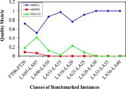
Quality metric versus classes of benchmarked instances
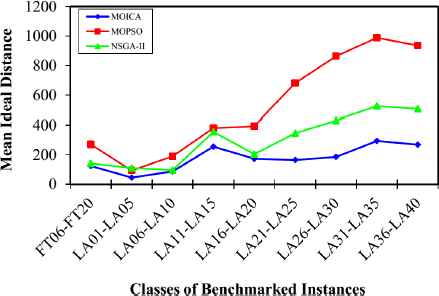
Mean ideal distance versus classes of benchmarked instances
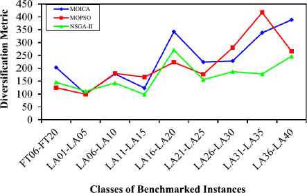
Diversification metric versus classes of benchmarked instances
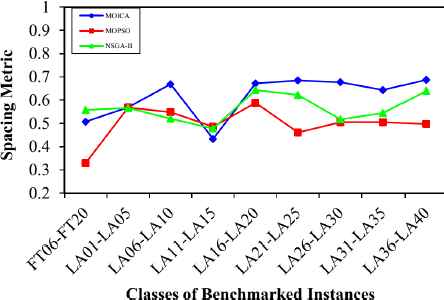
Spacing metric versus classes of benchmarked instances
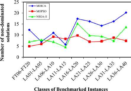
Number of non-dominated solutions versus classes of benchmarked instances
As illustrative examples, Figs. 15–18 present the non-dominated solutions of four test problems, LA25, LA32, LA36, and LA39, achieved by MOICA, MOPSO, and NSGA-II. The proposed MOICA is able to achieve high quality Pareto solutions, and they dominate a higher portion of the Pareto solutions obtained by the other approaches, as can be seen in Figs. 15–18. It is also clear that MOICA discovers more non-dominated solutions as compared to MOPSO and NSGA-II. Therefore, it is an efficient and powerful approach in finding more non-dominated solutions with higher quality. For illustration purposes, LA39 is randomly selected among the test problems, and one of its non-dominated solutions achieved by the proposed MOICA is depicted in Fig. 19.
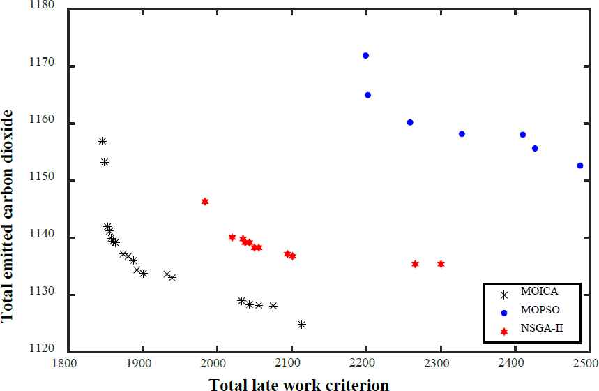
Non-dominated solutions of LA25 obtained by each algorithm
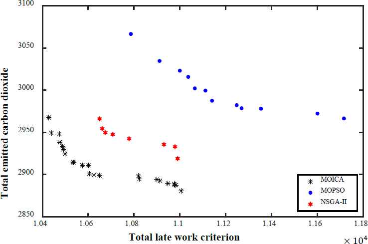
Non-dominated solutions of LA32 obtained by each algorithm
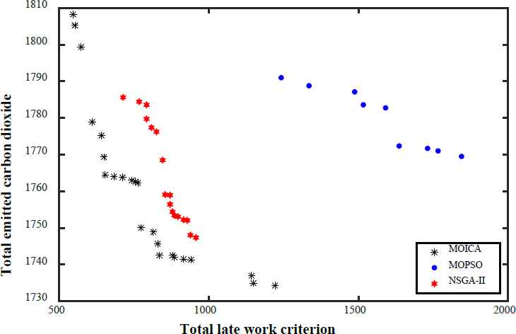
Non-dominated solutions of LA36 obtained by each algorithm
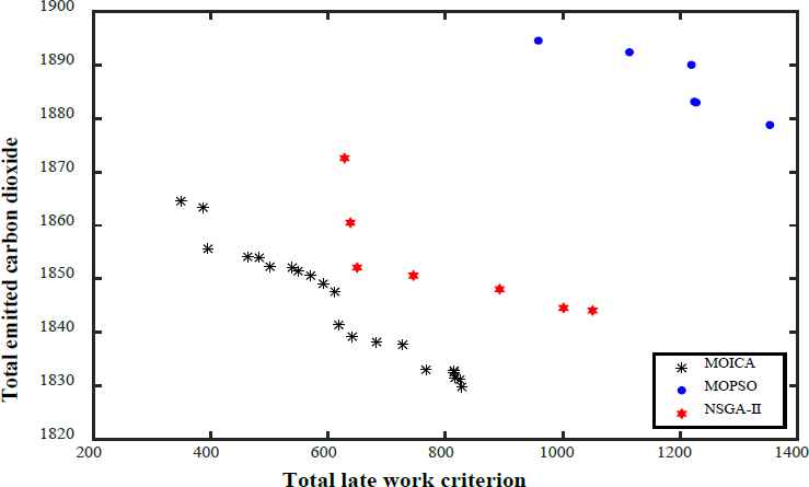
Non-dominated solutions of LA39 obtained by each algorithm
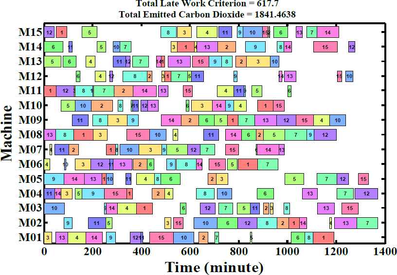
One of the non-dominated solutions of LA39 obtained by the proposed MOICA
It can be observed that MOICA contributes more high quality non-dominated solutions, that are better than most of the solutions discovered by the other algorithms. The achieved non-dominated solutions of MOICA generally have a lower MID in comparison to those of MOPSO and NSGA-II; that is, in most cases, the non-dominated solutions of MOICA have a lower distance from the optimal points in comparison to the other algorithms. In the proposed MOICA, the average value of DM is higher in comparison to those of the other approaches, i.e. the boundaries of non-dominated solutions discovered by MOICA are bigger in most of the test problems in comparison to MOPSO and NSGA-II.
5.5. Implications
The main focus of an eco-efficient-based multi-objective scheduling problem is to optimize environmental performance measures (eco-efficient-based objective functions) while improving customer satisfaction and efficiency (classical-based objective functions) throughout the scheduling period. In this research, the eco-efficient-based performance measure was optimized by considering power consumption of machines in different states (either busy or idle state). In order to utilize the proposed MOICA, certain initial input data such as the number of jobs, number of machines, technological sequence of operations for each job, processing time of each operation, due date of each job, and power consumption of each machine need to be entered into the algorithm. The proposed MOICA searches for a set of optimized non-dominated schedules, where different operations of jobs are optimally sequenced in a proper order on known machines. One of these high quality non-dominated schedules that is practically feasible can be adopted in a job shop scheduling environment. Based on the selected schedule from amongst the non-dominated schedules, managers can obtain useful information such as the start time of each operation, start time of each machine, idle duration of each machine, completion time of each operation, and completion time of each machine.
Moreover, additional managerial information with regard to the relationship between carbon footprint and total late work criterion can be derived, and this information can be used while weighing up these two objective functions in order to select a schedule from amongst a set of non-dominated schedules. It is noted that managerial and enterprise policies affect the priorities which could have been given to each of the objective functions. Based on the computational outcomes, the proposed MOICA is able to produce a higher number of high quality non-dominated schedules as compared to MOPSO and NSGA-II. Therefore, depending upon the managerial and enterprise policies in weighing up the objective functions, managers have the flexibility to determine the best schedule from amongst a set of non-dominated schedules.
6. Conclusions
In this paper, a new low-carbon based multi-objective job shop scheduling problem was introduced in which the objectives were to minimize carbon footprint and total late work criterion, simultaneously. Then, a new MOICA was developed to solve the presented problem. Forty-three test problems were solved by the proposed algorithm. Numerical results and comparison metrics showed the effectiveness of the proposed algorithm in comparison to MOPSO and NSGA-II for solving these test problems. To the best of the authors’ knowledge, this work is the first that considers the green and low-carbon job shop scheduling problems. It is also the first work that considers the total late work criterion in multi-objective job shop scheduling problems, and it is the pioneer paper that solves these problems by using MOICA. This work can be considered as an important addition to the literature, where the majority of the research papers have neglected green and low-carbon objectives. As extensions of this work, future studies can focus on other scheduling objectives such as makespan, tardiness, earliness, and buffer size while considering environmental objectives such as carbon emission and water scarcity. It is also interesting to apply other novel metaheuristic approaches in order to obtain more optimized solutions.67, 68
Acknowledgements
The authors would like to thank the Ministry of Higher Education (MOHE) and University Technology Malaysia (UT) for supporting this research (Vote Number: 4F840).
Appendix A.
See Table A1.
| Instance Name | Size | M1 | M2 | M3 | M4 | M5 | M6 | M7 | M8 | M9 | M10 | M11 | M12 | M13 | M14 | M15 |
|---|---|---|---|---|---|---|---|---|---|---|---|---|---|---|---|---|
| FT 06 | 6×6 | 11.21 | 6.74 | 8.5 | 5.3 | 6.55 | 8.64 | - | - | - | - | - | - | - | - | - |
| FT 10 | 10×10 | 10.55 | 16 | 17.24 | 11.1 | 13.51 | 8.18 | 8.25 | 13.37 | 16.16 | 11.88 | - | - | - | - | - |
| FT 20 | 20×5 | 9.79 | 7.21 | 12.07 | 5.13 | 14.39 | - | - | - | - | - | - | - | - | - | - |
| LA 01 | 10×5 | 10.01 | 13.53 | 17.22 | 15.37 | 15.16 | - | - | - | - | - | - | - | - | - | - |
| LA 02 | 10×5 | 16.14 | 10.1 | 10 | 6.18 | 14.89 | - | - | - | - | - | - | - | - | - | - |
| LA 03 | 10×5 | 8.23 | 14.81 | 5.18 | 6.62 | 17.22 | - | - | - | - | - | - | - | - | - | - |
| LA 04 | 10×5 | 13.15 | 7.39 | 10.6 | 11.45 | 11.04 | - | - | - | - | - | - | - | - | - | - |
| LA 05 | 10×5 | 17.43 | 15.59 | 14.48 | 10.95 | 11.58 | - | - | - | - | - | - | - | - | - | - |
| LA 06 | 15×5 | 14.25 | 14.09 | 12.89 | 11.74 | 11.62 | - | - | - | - | - | - | - | - | - | - |
| LA 07 | 15×5 | 17.27 | 12.8 | 14.46 | 6.79 | 14.89 | - | - | - | - | - | - | - | - | - | - |
| LA 08 | 15×5 | 14.63 | 17.56 | 5.78 | 6.71 | 5.98 | - | - | - | - | - | - | - | - | - | - |
| LA 09 | 15×5 | 14.37 | 15.79 | 10.63 | 9.92 | 5.43 | - | - | - | - | - | - | - | - | - | - |
| LA 10 | 15×5 | 17.01 | 13.67 | 6.92 | 7.56 | 16.92 | - | - | - | - | - | - | - | - | - | - |
| LA 11 | 20×5 | 5.65 | 13.79 | 5.73 | 12.21 | 13.26 | - | - | - | - | - | - | - | - | - | - |
| LA 12 | 20×5 | 11.25 | 7.67 | 17.17 | 17.28 | 16.64 | - | - | - | - | - | - | - | - | - | - |
| LA 13 | 20×5 | 5.85 | 15.54 | 8.04 | 11.41 | 11.36 | - | - | - | - | - | - | - | - | - | - |
| LA 14 | 20×5 | 7.92 | 14.15 | 17.58 | 9.63 | 7.64 | - | - | - | - | - | - | - | - | - | - |
| LA 15 | 20×5 | 7.89 | 9.77 | 8 | 12.51 | 11.86 | - | - | - | - | - | - | - | - | - | |
| LA 16 | 10×10 | 5.38 | 9.91 | 16.16 | 7.13 | 7.83 | 7.03 | 16.99 | 8.08 | 15.28 | 10.98 | - | - | - | - | - |
| LA 17 | 10×10 | 12.7 | 6.07 | 6.87 | 7.83 | 17.19 | 15.33 | 15.25 | 14.23 | 6.83 | 10.3 | - | - | - | - | - |
| LA 18 | 10×10 | 10.58 | 5.48 | 12.08 | 16.65 | 16.51 | 14.22 | 5.36 | 7.43 | 15.85 | 11.42 | - | - | - | - | - |
| LA 19 | 10×10 | 6.94 | 9.69 | 13.24 | 11.45 | 13.04 | 13.09 | 13.16 | 15.15 | 13.51 | 11.87 | - | - | - | - | - |
| LA 20 | 10×10 | 11.25 | 13.76 | 16.09 | 16.53 | 5.31 | 13.73 | 5.5 | 17.45 | 10.51 | 6.43 | - | - | - | - | - |
| LA 21 | 15×10 | 15.43 | 9.61 | 9.33 | 14.88 | 13.99 | 7.26 | 7.5 | 17.45 | 6.29 | 5.55 | - | - | - | - | - |
| LA 22 | 15×10 | 11.32 | 14.36 | 7.77 | 12.73 | 12.15 | 8.2 | 5.54 | 6.11 | 9.26 | 17.67 | - | - | - | - | - |
| LA 23 | 15×10 | 14.88 | 14.97 | 5.81 | 10.67 | 13.88 | 10.3 | 9.75 | 7.89 | 5.54 | 6.25 | - | - | - | - | - |
| LA 24 | 15×10 | 15.63 | 16.45 | 13.46 | 13.04 | 9.66 | 5.65 | 11.61 | 15.55 | 12.7 | 14.62 | - | - | - | - | - |
| LA 25 | 15×10 | 6.8 | 7.9 | 16.57 | 15.54 | 13.9 | 10.6 | 15.67 | 9.21 | 5.21 | 5.67 | - | - | - | - | - |
| LA 26 | 20×10 | 13.25 | 14.48 | 7.9 | 6.43 | 17.92 | 17.74 | 9.3 | 5.18 | 15.65 | 9.32 | - | - | - | - | - |
| LA 27 | 20×10 | 7.94 | 5.26 | 6.76 | 12.51 | 10.8 | 17.35 | 12.77 | 16.16 | 5.66 | 17.33 | - | - | - | - | - |
| LA 28 | 20×10 | 15.1 | 12.61 | 9.53 | 14.71 | 11.68 | 5.51 | 9.41 | 13.49 | 6.96 | 6.31 | - | - | - | - | - |
| LA 29 | 20×10 | 7.12 | 13.74 | 16.55 | 14.74 | 17.79 | 11.73 | 9.76 | 6.16 | 17.23 | 13.11 | - | - | - | - | - |
| LA 30 | 20×10 | 11.4 | 10.48 | 12.88 | 14.16 | 14.94 | 14.79 | 16.82 | 17.09 | 8 | 8.17 | - | - | - | - | - |
| LA 31 | 30×10 | 15.92 | 8.41 | 17.34 | 12.33 | 13.43 | 13.44 | 17.34 | 14.87 | 12.64 | 6.08 | - | - | - | - | - |
| LA 32 | 30×10 | 8.38 | 15.18 | 13.92 | 7.2 | 15.66 | 17.05 | 11.38 | 14.51 | 16.27 | 6.43 | - | - | - | - | - |
| LA 33 | 30×10 | 16.73 | 8.36 | 6.88 | 8.4 | 14.88 | 16.81 | 10.57 | 14.48 | 11.49 | 15.57 | - | - | - | - | - |
| LA 34 | 30×10 | 9.96 | 5.68 | 15.93 | 13.71 | 5.61 | 17.3 | 5.93 | 7.91 | 12.73 | 9.49 | - | - | - | - | - |
| LA 35 | 30×10 | 5.56 | 8.56 | 7.44 | 14.43 | 14.9 | 16.16 | 14.69 | 6.47 | 7.66 | 16.14 | - | - | - | - | - |
| LA 36 | 15×15 | 12.36 | 11.25 | 7.68 | 14.19 | 8.74 | 14.04 | 13.87 | 11.31 | 9.48 | 7.9 | 10.04 | 9.78 | 7.9 | 14.21 | 6.78 |
| LA 37 | 15×15 | 12.15 | 5.31 | 5.44 | 7.88 | 11.63 | 16.89 | 6.11 | 11.82 | 14.95 | 12.91 | 14.98 | 9.19 | 12.72 | 17.26 | 13.43 |
| LA 38 | 15×15 | 8.46 | 13.36 | 7.36 | 13.71 | 15.33 | 17.03 | 10.6 | 16.07 | 8.77 | 8.04 | 15.19 | 13.91 | 9.73 | 12.51 | 10.23 |
| LA 39 | 15×15 | 9.68 | 17.05 | 10.78 | 14.4 | 8.95 | 6.56 | 16.06 | 9.52 | 15.64 | 17.28 | 9.79 | 6.73 | 10.47 | 9.53 | 8.98 |
| LA 40 | 15×15 | 17.53 | 13.88 | 15 | 9.47 | 8.37 | 14.52 | 14.79 | 6.41 | 6.24 | 5.06 | 11.09 | 12.89 | 15.93 | 13.79 | 11.68 |
Power consumption data in processing state (Power in kW)
Appendix B.
See Table B1.
| Instance Name | Size | M1 | M2 | M3 | M4 | M5 | M6 | M7 | M8 | M9 | M10 | M11 | M12 | M13 | M14 | M15 |
|---|---|---|---|---|---|---|---|---|---|---|---|---|---|---|---|---|
| FT 06 | 6×6 | 1.53 | 2.13 | 2.66 | 1.32 | 1.04 | 2.33 | - | - | - | - | - | - | - | - | - |
| FT 10 | 10×10 | 2.2 | 1 | 1.75 | 1.23 | 2.06 | 1.6 | 1.31 | 2.15 | 2.14 | 1.96 | - | - | - | - | - |
| FT 20 | 20×5 | 1.34 | 1.05 | 2.83 | 2.62 | 1.76 | - | - | - | - | - | - | - | - | - | - |
| LA 01 | 10×5 | 2.19 | 2.42 | 2.54 | 1.8 | 2.51 | - | - | - | - | - | - | - | - | - | - |
| LA 02 | 10×5 | 1.95 | 1.21 | 2.04 | 2.19 | 1.15 | - | - | - | - | - | - | - | - | - | - |
| LA 03 | 10×5 | 1.59 | 2.91 | 1.67 | 1.22 | 1.96 | - | - | - | - | - | - | - | - | - | - |
| LA 04 | 10×5 | 2.03 | 2.68 | 2.9 | 2.48 | 2.07 | - | - | - | - | - | - | - | - | - | - |
| LA 05 | 10×5 | 2.43 | 1.02 | 2.2 | 2.09 | 2.27 | - | - | - | - | - | - | - | - | - | - |
| LA 06 | 15×5 | 2.34 | 1.23 | 2.89 | 2.65 | 2.51 | - | - | - | - | - | - | - | - | - | - |
| LA 07 | 15×5 | 2.17 | 2.29 | 1.98 | 1.82 | 1.57 | - | - | - | - | - | - | - | - | - | - |
| LA 08 | 15×5 | 2.11 | 2.35 | 2.97 | 2.52 | 2.04 | - | - | - | - | - | - | - | - | - | - |
| LA 09 | 15×5 | 2.48 | 1.53 | 2.85 | 1.01 | 1.11 | - | - | - | - | - | - | - | - | - | - |
| LA 10 | 15×5 | 2.59 | 1.88 | 1.99 | 1.54 | 1.4 | - | - | - | - | - | - | - | - | - | - |
| LA 11 | 20×5 | 1.96 | 1.8 | 2.75 | 2.6 | 2.73 | - | - | - | - | - | - | - | - | - | - |
| LA 12 | 20×5 | 1.16 | 2.96 | 1.65 | 2.43 | 1.56 | - | - | - | - | - | - | - | - | - | - |
| LA 13 | 20×5 | 2.8 | 2.94 | 2.02 | 2.61 | 2.58 | - | - | - | - | - | - | - | - | - | - |
| LA 14 | 20×5 | 1.14 | 1.65 | 1.36 | 2.22 | 2.88 | - | - | - | - | - | - | - | - | - | - |
| LA 15 | 20×5 | 1.2 | 2.29 | 1.75 | 1.52 | 1.61 | - | - | - | - | - | - | - | - | - | - |
| LA 16 | 10×10 | 1.75 | 2.31 | 1.02 | 2.78 | 1.79 | 2.29 | 1.47 | 1.17 | 2.72 | 2.67 | - | - | - | - | - |
| LA 17 | 10×10 | 2.2 | 2.27 | 2.49 | 1.37 | 2.57 | 2.94 | 1.09 | 2.95 | 2.84 | 1.01 | - | - | - | - | - |
| LA 18 | 10×10 | 1.96 | 2.99 | 2.2 | 2.68 | 1.26 | 2.41 | 1.33 | 2.71 | 1.58 | 1.57 | - | - | - | - | - |
| LA 19 | 10×10 | 2.27 | 1.41 | 2.43 | 1.13 | 1.36 | 1.98 | 2.55 | 2.76 | 1.33 | 2.9 | - | - | - | - | - |
| LA 20 | 10×10 | 2.52 | 1.44 | 2.46 | 1.15 | 2.49 | 1.65 | 1.07 | 1.27 | 2.41 | 2.65 | - | - | - | - | - |
| LA 21 | 15×10 | 1.04 | 2.94 | 1.1 | 1.08 | 2.2 | 2.54 | 2.77 | 2.06 | 2.72 | 1.1 | - | - | - | - | - |
| LA 22 | 15×10 | 2.4 | 2.08 | 2.41 | 2.98 | 2.31 | 1.04 | 1.13 | 2.98 | 1.68 | 2.26 | - | - | - | - | - |
| LA 23 | 15×10 | 1.08 | 1.44 | 2.7 | 2.1 | 1.23 | 2.27 | 1.07 | 2.11 | 2.98 | 1.48 | - | - | - | - | - |
| LA 24 | 15×10 | 2.65 | 2.19 | 1.34 | 1.39 | 2.92 | 2.64 | 2.9 | 1.97 | 1.46 | 1.96 | - | - | - | - | - |
| LA 25 | 15×10 | 2.41 | 2.62 | 2.78 | 1.53 | 2.59 | 1.46 | 1.08 | 1.22 | 2.64 | 1.71 | - | - | - | - | - |
| LA 26 | 20×10 | 2.13 | 2.8 | 1.09 | 1.29 | 2.29 | 2.66 | 2.24 | 2.95 | 2.25 | 2.46 | - | - | - | - | - |
| LA 27 | 20×10 | 1.11 | 1.01 | 2.69 | 1.21 | 2.38 | 2.07 | 1.9 | 1.92 | 1.99 | 1.19 | - | - | - | - | - |
| LA 28 | 20×10 | 1.65 | 2.12 | 2.37 | 2.43 | 1.93 | 1.24 | 1.32 | 2.69 | 1.68 | 1.52 | - | - | - | - | - |
| LA 29 | 20×10 | 1.57 | 2.1 | 1.51 | 2.35 | 1.48 | 2.58 | 2.16 | 1.22 | 1.8 | 2.58 | - | - | - | - | - |
| LA 30 | 20×10 | 1.83 | 1.12 | 1.66 | 2.2 | 2.94 | 2.66 | 1.2 | 1.39 | 2.08 | 1.43 | - | - | - | - | - |
| LA 31 | 30×10 | 2.11 | 2.48 | 2.31 | 2.31 | 1.54 | 2.65 | 2.73 | 1.27 | 1.5 | 1.82 | - | - | - | - | - |
| LA 32 | 30×10 | 2.03 | 2.2 | 2.43 | 1.14 | 1.67 | 2.38 | 2.37 | 2.91 | 2.75 | 2.28 | - | - | - | - | - |
| LA 33 | 30×10 | 2.22 | 1.04 | 1.85 | 1.98 | 2.33 | 2.83 | 1.79 | 2.84 | 2.24 | 2.87 | - | - | - | - | - |
| LA 34 | 30×10 | 2.82 | 1.15 | 1.76 | 1.5 | 1.59 | 1.94 | 1 | 1.86 | 1.89 | 2.76 | - | - | - | - | - |
| LA 35 | 30×10 | 1.71 | 2.93 | 2.14 | 2.81 | 1.99 | 2.23 | 2.71 | 1.17 | 1.47 | 2.38 | - | - | - | - | - |
| LA 36 | 15×15 | 1.52 | 1.41 | 2.59 | 1.31 | 1.65 | 1.67 | 2.95 | 1.13 | 2.07 | 2.59 | 1.16 | 1.24 | 1.06 | 2.11 | 1.49 |
| LA 37 | 15×15 | 1.85 | 1.29 | 2.06 | 2.55 | 2.75 | 1.31 | 2.77 | 1.11 | 1.82 | 1.02 | 1.77 | 2.05 | 2.44 | 2.69 | 1.59 |
| LA 38 | 15×15 | 1.34 | 1.53 | 1.91 | 1.28 | 2.02 | 2.4 | 1.26 | 2.79 | 2.79 | 1.54 | 1.35 | 2.37 | 1.17 | 1.83 | 1.82 |
| LA 39 | 15×15 | 1.51 | 2.22 | 1.01 | 2.46 | 2.22 | 1.13 | 1.99 | 2.81 | 1.29 | 2.01 | 2.03 | 1.25 | 2.43 | 2.54 | 1.1 |
| LA 40 | 15×15 | 1.55 | 2.76 | 1.05 | 1.38 | 1.54 | 1.16 | 1.96 | 1.72 | 1.39 | 1.41 | 2.69 | 1.99 | 1.87 | 2.73 | 1.35 |
Power consumption data in idle state (Power in kW)
References
Cite this article
TY  - JOUR
AU  - Hamed Piroozfard
AU  - Kuna Yew Wong
AU  - Manor Kumar Tiara
PY  - 2018
DA  - 2018/01/01
TI  - Reduction of carbon emission and total late work criterion in job shop scheduling by applying a multi-objective imperialist competitive algorithm
JO  - International Journal of Computational Intelligence Systems
SP  - 805
EP  - 829
VL  - 11
IS  - 1
SN  - 1875-6883
UR  - https://doi.org/10.2991/ijcis.11.1.62
DO  - 10.2991/ijcis.11.1.62
ID  - Piroozfard2018
ER  -