
An Agile Mortality Prediction Model: Hybrid Logarithm Least-Squares Support Vector Regression with Cautious Random Particle Swarm Optimization
- DOI
- 10.2991/ijcis.11.1.66How to use a DOI?
- Keywords
- intensive care; mortality prediction; logarithm least-squares support vector regression; cautious random particle swarm optimization
- Abstract
Logarithm Least-Squares Support Vector Regression (LLS-SVR) has been applied in addressing forecasting problems in various fields, including bioinformatics, financial time series, electronics, plastic injection moulding, Chemistry and cost estimations. Cautious Random Particle Swarm Optimization (CRPSO) uses random values that allow pbest and gbest to be adjusted to the correct weight using a random value. CRPSO limits the random value to be conditional, to avoid premature convergence into a local optimum. If the random value is greater than 0.6, another random value is chosen. The movement of the range (cautious flow) is controlled to avoid premature convergence. This pilot study retrospectively collected data on 695 patients admitted to intensive care units and constructed a novel mortality prediction model with logarithm least-squares support vector regression (LLS-SVR) and cautious random particle swarm optimization (CRPSO). LLS-SVR-CRPSO was employed to optimally select the parameters of the hybrid system. This new mortality model can offer agile support for physicians’ intensive care decision-making.
- Copyright
- © 2018, the Authors. Published by Atlantis Press.
- Open Access
- This is an open access article under the CC BY-NC license (http://creativecommons.org/licences/by-nc/4.0/).
1. Introduction
Intensive care is one of the most important components in modern health care systems, and outcome evaluation of patients is a key component of intensive care facility allocation decisions [1]. In order to achieve optimal facility allocation, some studies have proposed the use of mortality prediction models as outcome predictors for intensive care patients. Several mortality prediction models have demonstrated high efficiency in this field, including the Acute Physiology and Chronic Health Evaluation System, 2nd version (APACHE II) [2], 3rd version (APACHE III) [3], 4th version (APACHE IV) [4], the Simplified Acute Physiology System, 2nd version (SAPS II) [5] and 3rd version [6], The Mortality Probability Model 2nd version (MPM II) [7] and 3rd version (MPM III) [8, 9].
There are several approaches in mortality prediction model construction. The first approach focuses on the tendency of mortality. McCabe and Jackson constructed the first mortality prediction model. They collected 173 septicemia patients and divided patients into nonfatal, ultimately fatal and fatal groups. The mortality rates of these groups were 11%, 66% and 91%, respectively. This model is thus able to calculate a tendency of mortality [10]. Cullen et al. collected 70 variables of patients and scored these variables from 1 to 4 with the tendency of severity. They evaluated the severity of patients with the summation of the collected scores. This was called the Therapeutic Intervention Scoring System (TISS) [11]. The models of this stage are the tendency of severity for patients. The Glasgow Coma Scale (GCS) is also a severity tendency model [12, 13]. These models focused on the tendency of mortalities based purely on a scoring system, rather than on a probability system.
The second approach is the probability approach. The two most popular models in this category are APACHE II and SAPS II [2,3, 14]. These models were constructed with probity regression, and used probabilities as the outcome description of mortality. The Mortality Probability Model 2nd version (MPM II) is also a probability-based ICU outcome prediction model [7]. This model was used to calculate the outcome probabilities of patients with their data within one hour of ICU admission. These models described the tendency of mortalities with probabilities, and new versions of these models have been constructed in recent studies [3, 4, 6].
Artificial intelligence technologies have since been built into mortality prediction models, and form the basis of the information technology approach. These models are more accurate than the traditional models [15, 16]. Support Vector Machine (SVM) was initially a form of information technology used in classification problems. It used both statistical learning and structural risk minimization to find an optimal separation hyper plane to separate different class outcomes in a multidimensional space [17, 18]. SVM solved many problems in different fields, included text categorization, image recognition, face detection, voice recognition, genetic classification and medical diagnostic problems [18–22]. Zhu et al. constructed SVM-based classifiers, which had better performance in evaluating the malignance of pulmonary nodules found in computer tomography [23]. Yamamoto et al. used SVM technology to correctly identify possible multiple sclerosis lesions in brain magnetic resonance images [22]. SVM technologies are good classification methods.
The PSO–SVM model combines PSO and SVM by using PSO to search SVM parameters [24]. The PSO–SVM model achieves higher accuracy than the BP NN model. The results obtained using the PSO–SVM method yield higher detection rates than regular SVM algorithms. PSO was applied to search the parameter C and the kernel function parameters gamma (γ) in the radial basis function (RBF) kernel [25]. Cautious random particle swarm optimization (CRPSO) used random design values that allow pbest and gbest to be adjusted to the correct weight using a random value. CRPSO limits the random value to be conditional, to avoid premature convergence into a local optimum. If the random value is greater than 0.6, another random value is chosen. The movement of the range (cautious flow) is controlled to avoid premature convergence.
This pilot study retrospectively collected data on 695 patients admitted to intensive care units and constructed a novel mortality prediction model with logarithm least-squares support vector regression (LLS-SVR) technologies and cautious random particle swarm optimization (CRPSO)[26]. LLS-SVR-CRPSO was employed to optimally select the parameters of the hybrid system. This new mortality model is able to offer agile support to physicians’ intensive care decision-making.
This paper has introduced traditional mortality prediction models, SVM, PSO, least-squares support vector regression (LS-SVR), logarithm least-squares support vector regression (LLS-SVR), and cautious random particle swarm optimization (CRPSO). Section 2 offers a brief review of logarithm least-squares support vector regressions (LLS-SVR), particle swarm optimization (PSO) cautious random particle swarm optimization (CRPSO) and parameter selection. In Section 3, the proposed method is used to model a nonlinear system in simulation and compared to current methods. Finally, Section 4 gives a summary of the work, and concluding remarks.
2. MATERIAL AND METHODS
2.1 Logarithm least-squares support vector regressions
The support vector machine model has been successfully extended for dealing with non-linear regression problems [1]. LS-SVR has also been used successfully for regression problems [27] and differs from SVR, which attempts to minimize SSEs of training data sets while simultaneously minimizing the margin error [1]. Moreover, Lin [28] first proposed logarithm support vector regression (LSVR) which has been demonstrated to achieve better performance than traditional SVR in forecasting problems. Therefore, the logarithm least-squares support vector regression (LLS-SVR) approach is proposed and employed in this study to approximate an unknown function by a training data set {(xi, log(yti)), i=1, …, N}. The logarithm regression function can be formulated as Eq. (1). LLS-SVR introduces a least squares version to LSVR by formulating the regression problem as:
The Lagrangian was introduced as:
Any function that satisfies Mercer’s condition [24] can act as the kernel function. Kernel functions enable the dot product to be computed in a high-dimension feature space using low-dimension data input without a transfer (φ) [1]. Note that in the case of the radial basis function (RBF) kernels which are represented in Eq. (6), one has only two additional tuning parameters (C,σ), which is less than that of a standard SVR.
2.2 Particle swarm optimization
Kennedy and Eberhart first proposed particle swarm optimization (PSO) in 1995. PSO simulates social behavior such as birds flocking and fish schooling. It is an emerging population-based meta-heuristic and a population based evolutionary algorithm to achieve precise objectives in a multidimensional space. A population (called a swarm) is made up of individuals (called particles) that are updated by iteration. All particles find the global optimum by moving in the problem space at each iteration. Each particle accords its own best previous experience and the best experience of all other members to correct the search direction. Two important factors are pbest and gbest, as when birds or fish determine their velocities by their own best previous experience (pBest) and the best experience of all other members (gBest) Eberhart and Kennedy [29], [30–32]. PSO is similar to genetic algorithm (GA), which is initialized with a population of random solutions [33]. However, PSO is used less frequently than GAs for computation time and setting parameters. PSO results can, however, easily be optimized if parameter values are set.
The particles are manipulated according to the following equation:
Vid is the rate of the position change (velocity) for particle I,
Xid is the ith particle,
C1 is the cognition learning factor,
C2 is the social learning factor,
Pid is its previous best position
Pgd is the global best positiont
Rand() and Rand() are two random functions in the range[26, 32, 34].
Yuhui Shi and Russell Eberhart used a new parameter, called inertia weight, to improve the performance of the particle swarm optimizer.[34] The new parameter w plays the role of balancing the global search and local search. The new equation as follow:
The pseudo code of the procedure is as follows:
Initialize location and velocity of each particle repeat
For each particle
Calculate fitness value
If the fitness value is better than the best fitness value
(pBest) in history
set current value as the new pBest
End
Choose the particle with the best fitness value of all the particles as the gBest
For each particle
Calculate particle velocity according equation (Eq.7)
Update particle position according equation (Eq.8)
End
until stopping criterion is met
2.3 Cautious Random Particle swarm optimization
PSO studies fall into three categories. The first determines inertia, and adjusts it in order to avoid falling into a local optimum, and increases the speed of convergence [35–38]. Some studies have dynamically adjusted the inertia in each iteration [39, 40].
The second category uses constriction factors C1 and C2 [41]. Studies have used the same or different weightings for individual optimal solutions (pbest) and the global optimal solution (gbest).
The third category adds other influencing factors to the best personal experience (pbest) and the best experience of the group (gbest) [42].
However, no studies have used random design values that allow pbest and gbest to be adjusted to the correct weight using a random value. Cautious Random Particle swarm optimization (CRPSO) limits the random value to be conditional, to avoid premature convergence into a local optimum[26]. If the random value is greater than o.8, another random value is chosen. The movement of the range (cautious flow) is controlled to avoid premature convergence (Figure 1).
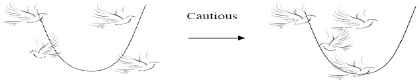
A Cautious flow
This study proposes that if a prescribed probability is used to adjust the random value, the algorithm is prevented from prematurely falling into a local optimum, and the convergence speed and search performance are improved. The procedure for the new algorithm is as follows:
- Step 1:
Generate the initial population. The population is generated randomly in the search space.
- Step 2:
Evaluate the population. The objective function value is considered as the fitness.
- Step 3:
If the fitness value is better than the best fitness value (pBest) in the history, set the current value as the new pBest.
- Step 4:
Choose the particle with the best fitness value of all the particles as the gBest
- Step 5:
If random value is greater than 0.8, then choose another random value
- Step 6:
Calculate the particle velocity, using equation (Eq. 3)
Update the particle position, using equation (Eq. 4) Then go to Step 2, until the stop criterion is met
This model adjusts the scales of randomization. It is found that a larger scale of randomization increases the possibility of premature convergence. Performance is increased if the random processes has “narrow/small steps” that are less than 0.6. ANOVA is used in this study to explain that different random values (0.6, 0.7, 0.8, 0.9) yield no significant difference [26] This randomization processes is called Cautious Random (CR). The study proposes that, given a prescribed probability that is adjusted randomly, the algorithm is prevented from prematurely falling into a local optimum, and the convergence speed and search performance are both improved. This concept is similar to that of mutation in a genetic algorithm. However CR involves inverse computing. Mutation significantly changes populations, while CR changes swarms cautiously. CRPSO thus performs better, because it prevents premature convergence and allows faster optimization.
2.4 Parameter selection
Suitable parameters will effectively improve the performance of LLS-SVR. Studies have adopted various algorithms to search SVR/LS-SVR parameters [43–45], and PSO has been a popular method for selecting parameters. This study, however, replaces PSO with CRPSO (Figure 2).
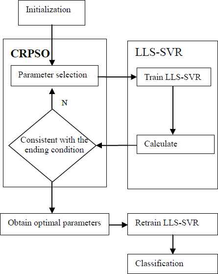
Flowchart of LLS-SVR-CRPSO
The operations of CRPSO are described in the LLS-SVR-CRPSO model as follows:
- Step 1
(Initialization). Initialize location and velocity of each particle.
- Step 2
(Evaluate fitness). In this study, a negative J is adopted as the fitness function.
where M is the number of forecasting periods, YCt is the actual value, and YC (xt) is the forecasting value at period t. - Step 3
(pBest). If the fitness value is better than the best fitness value (pBest) in the history, set current value as the new pBest.
- Step 4
(gBest). Choose the particle with the best fitness value of all particles as the gBest.
- Step 5:
If random value is greater than 0.8, then choose another random value
- Step 6
(Next generation). Form a population for the next generation.
- Step 7
(Stop condition). If the number of generations equals a given scale, present the best as a solution; otherwise go back to Step 2.
3. Numerical examples and experimental results
3.1 Patients profiles
This study retrospectively collected training data from 695 patients (230 women and 465 men) who were admitted to the surgical ICU in a 600-bed hospital (12-bed surgical ICU) from January 1, 2000 to December 31, 2006. All patients’ data were collected confidentially with randomized codes. The average patient age was 57.26 (SD=20.41) years.
The attributes are shown in table 1. The age, type of admission (medical diseases, elective and emergency surgery) and Glasgow coma scale (GCS) (table 2) are all included in the attributes. The scale consists of three separate responses: eye opening, verbal and motor responses, each classified by a series of grades of responsiveness. Each subdivision of responsiveness can be allocated a number, better grades scoring higher. The score of eye opening (GCS eye) is 1 to 4. The score of best verbal response (GCS verbal) is 1 to 5. The score of best motor response (GCS motor) is 1 to 6.The definition of “alive” indicates that patients were discharged alive or stayed in hospital for at least 30 days. The definition of dead is that the patients died during treatment.
| Independent variables | Mean | SD |
|---|---|---|
| Body Temperature (°C) | 36.51 | 1.78 |
| Systolic BP (mmHg) | 138.7 | 35.6 |
| Diastolic BP (mmHg) | 75.5 | 21.0 |
| Heart Rate (per min) | 100.5 | 24.8 |
| Breath Rate (per min) | 19.669 | 5.875 |
| Urine output (c.c.) | 3383 | 4732 |
| Bilirubin (mg/dL) | 0.45 | 1.48 |
| Sodium (mEq/L) | 141.6 | 10.3 |
| Potasium (mEq/L) | 3.81 | 0.74 |
| Blood urine nitrogen (mg/dL) | 18.09 | 17.62 |
| Creatinine (mg/dL) | 1.2 | 1.1 |
| Sugar (mg/dL) | 147.8 | 73.4 |
| Hematocrit (%) | 33.30 | 6.50 |
| WBC (/ul) | 11251 | 5278 |
| Arterial pH | 7.399 | 0.098 |
| HCO3 (mEq/L) | 22.73 | 4.64 |
| PaO2 | 146.3 | 85.7 |
Patient attributes and information
| Score | GCS eye | GCS verbal | GCS motor |
|---|---|---|---|
| 1 | Never (172) | None (347) | No response (99) |
| 2 | To Pain (58) | Incomprehensible (20) | Extension (45) |
| 3 | To sound (142) | Inappropriate (16) | Flexion: abnormal (20) |
| 4 | Spontaneou (323) | Confused (40) | Flexion: normal (45) |
| 5 | Orientated (272) | Localize (136) | |
| 6 | Obey commands (350) | ||
| Total | 695 | 695 | 695 |
The case numbers of the Glasgow coma scale
3.2 Result
This study adopts four forecasting models, SVM, LLSVR-GA and LLS-SVRPSO to demonstrate the superiority of the proposed LLS-SVRPSO model. The logarithm LLSSVR-GA has been proposed to improve the performance of SVM by logarithm function [28]. Therefore, LLS-SVR-CRPSO is designed and examined in the example in the research.
Table 3 shows the forecasting performances of the four models and ranking in mortality forecasting data. Table 3 shows that the proposed LLS-SVR-PSO and LLSVRCRPSO models outperformed the other models in terms of forecasting accuracy because of their preprocess mechanisms. This demonstrates that the proposed LLS-SVR-PSO achieves superior performance. It can be seen that when the proposed and CRPSO models selected two parameters of LLSVR, their accuracy was the same. We used Matlab(2010b) to set 200 iterations each runtime. The random value of LLS-SVR-PSO is range [0,1]. The random value of LLS-SVR-CRPSO is greater than 0.6. Tables 4 and 5 show the results of 10 runs with the PSO and CRPSO models. The CRPSO model clearly has faster convergence than the PSO model. The average iteration of CRPSO is 86. The average iteration of PSO is 113. This is a significant improvement, because it is very important that physicians be provided with decision-making references as fast as possible in real emergency situations..
| Method | Accuracy rate | Rank |
|---|---|---|
| LLSVR-CRPSO | 0.85 | 1 |
| LLSVR-PSO | 0.85 | 2 |
| LLSVR-GA | 0.81 | 3 |
| SVM | 0.8 | 4 |
Comparison of three forecasting models
| Times | gam | sin2 | convergence (iteration) |
|---|---|---|---|
| 1 | 17.7967 | 379.4120 | 94* |
| 2 | 12.8673 | 527.2764 | 81 |
| 3 | 14.9415 | 1046.5419 | 80** |
| 4 | 17.2533 | 317.3528 | 81 |
| 5 | 7.7432 | 415.5156 | 94 |
| 6 | 22.1692 | 919.2539 | 87 |
| 7 | 17.247 | 370.4547 | 87 |
| 8 | 18.9399 | 487.5750 | 89 |
| 9 | 6.4584 | 695.4138 | 82 |
| 10 | 22.291 | 484.0880 | 85 |
| Average | 86 |
is the slowest iteration of convergence
is the fastest iteration of convergence
Convergence of LLS-SVR-CRPSO model
| Times | gam | sin2 | convergence (iteration) |
|---|---|---|---|
| 1 | 19.6689 | 444.5899 | 135* |
| 2 | 18.9136 | 635.2215 | 123 |
| 3 | 14.1529 | 1336.8530 | 122 |
| 4 | 9.4010 | 536.2189 | 100** |
| 5 | 24.5441 | 1620.0947 | 104 |
| 6 | 14.3800 | 335.9559 | 104 |
| 7 | 24.7495 | 832.1090 | 109 |
| 8 | 32.9367 | 1744.1732 | 101 |
| 9 | 14.4665 | 793.2447 | 122 |
| 10 | 13.9755 | 340.0115 | 116 |
| Average | 113 |
is the slowest iteration of convergence
is the fastest iteration of convergence
Convergence of LLS-SVR-PSO model
4. Conclusions
This study developed a novel LLS-SVR-CRPSO model for the prediction of mortality probabilities in intensive care units. Simultaneous results indicate that the LLS-SVR-CRPSO model offers a promising alternative for mortality forecasting. The superior performance of the LLS-SVR-CRPSO model can be ascribed to two causes. First, the LLS-SVR-CRPSO can efficiently capture trends of medical data. Second, the LLS-SVR-CRPSO with logarithm function mechanisms can effectively improve performance of predictions for mortality forecasting. This new mortality model can rapidly provide critical support information for physicians’ intensive care decision-making. Future work will use other ICU domain data sets or standard data sets to verify the superior performance of the proposed LLS-SVR-CRPSO model.
References
Cite this article
TY  - JOUR
AU  - Chien-Lung Chan
AU  - Chia-Li Chen
AU  - Hsien-Wei Ting
AU  - Dinh-Van Phan
PY  - 2018
DA  - 2018/01/01
TI  - An Agile Mortality Prediction Model: Hybrid Logarithm Least-Squares Support Vector Regression with Cautious Random Particle Swarm Optimization
JO  - International Journal of Computational Intelligence Systems
SP  - 873
EP  - 881
VL  - 11
IS  - 1
SN  - 1875-6883
UR  - https://doi.org/10.2991/ijcis.11.1.66
DO  - 10.2991/ijcis.11.1.66
ID  - Chan2018
ER  -