
A model-reference impedance control of robot manipulators using an adaptive fuzzy uncertainty estimator
- DOI
- 10.2991/ijcis.11.1.74How to use a DOI?
- Keywords
- model-reference; impedance control; electrically driven robot manipulators; fuzzy uncertainty estimator
- Abstract
This paper aims at developing a voltage-based impedance model-reference controller using fuzzy uncertainty estimator for the robust control of electrically driven robot manipulators. The proposed control scheme not only utilizes a desired impedance as a reference model, but also provides the integrated control of position and force in the closed loop system. The robotic system receives the output of model-reference as a desired trajectory and thus the aim of the controller is to reduce the difference between the task-space desired trajectory and the desired impedance model. Furthermore, two control terms namely a robustifying term and a fuzzy uncertainty estimator are added in the structure of control design in order to improve the performance of the control system as well as to tackle uncertainty including un-modelled dynamics and external disturbances. Using stability analysis, we derive the adaptive mechanisms and also prove the boundedness of all system states. Finally, simulation results are included to verify the proposed control method.
- Copyright
- © 2018, the Authors. Published by Atlantis Press.
- Open Access
- This is an open access article under the CC BY-NC license (http://creativecommons.org/licences/by-nc/4.0/).
1. Introduction
Many researchers have focused attention on designing force control schemes for robot manipulators in the past decades. As an end-effector of robot manipulators interacts with an environment, the existing contact force must be regulated to protect the end-effector and environment against serious damages. To solve this problem, the hybrid position/force control approaches [1–2] have been proposed to guarantee a smooth transition from position control to force control. However, the formulation of hybrid position/force control cannot be easily achieved. Also, many of these control schemes require the exact kinematics and dynamics of robotic system; hence, an adaptive Jacobian position/force control [3] has been developed which does not require all the knowledge of the robot manipulator.
In order to provide a unified solution of the position and force control, the impedance control schemes [4–6] have been developed for robot manipulators. An impedance model is designed to describe the dynamic behavior of a robotic system when interacting with the environment. It is worth noting that impedance control methods are strongly affected by the uncertainty associated with the nonlinear dynamics of highly coupled robotic systems, unknown environments and external disturbances [7]. Therefore, the performance of control system is dependent on how well the uncertainty can be compensated [8]. Adaptive impedance controllers [9], robust impedance controller [10], learning impedance control [11] and force tracking impedance control [12] have been developed to tackle uncertainty. It should be emphasized that the majority of impedance controllers are based on torque control strategy such that the proposed control laws require the dynamics of robot manipulator and also the role of robot's motors is excluded from the control problem.
To consider the whole robotic system including robot manipulator and motors, a regressor-based variable-structure controller [13], the min-max scheme [14] and a generalized impedance controller [15] have been proposed. By using the voltage control strategy [16–17], the impedance control of electrically driven robots has been proposed [18]. The main idea behind the voltage control strategy comes from the fact that the manipulator dynamics can be taken into account indirectly as measuring the motor currents.
An adaptive impedance control of human-robot cooperation [19] has been developed. In this control method, linear quadratic regulation has been formulated to minimize tracking errors and to obtain an optimal impedance mode of human. An adaptive neural impedance controller [20] for robot manipulators has been proposed by considering uncertainty and input saturation. An adaptive control method [21] has been designed for tracking purpose of uncertain robotics in order to compensate parametric uncertainties, unmodelled dynamics and external force disturbances without a priori knowledge about upper bound of uncertainty. An adaptive fuzzy neural network force approach [22], robust neural network [23] and robust adaptive neuro-fuzzy controller [24] for hybrid position/force control of robot manipulators have been developed, which interacts with unknown environment. A PID-fuzzy controller was developed to deal with the nonlinear contact force control problem [25].
This paper presents a voltage-based model-reference impedance control approach using a fuzzy uncertainty estimator for the electrically driven robot manipulators. In the proposed control scheme, a desired impedance is used as a model-reference in such a way that this model-reference could provide a reference signal for a robot in both tracking and contact situations. As the interaction between an end-effector and an environment occurs, the contact force is exerted to the model-reference and the robotic system receives the output of model-reference as a desired trajectory and thus the aim of the controller is to reduce the difference between the task-space desired trajectory and the desired impedance model. In order to tackle difficulties in the analysis of the motion equation in task-space, a specific transformation is used and a pertinent controller is designed in the joint-space. Furthermore, two control terms namely, a robustifying term and a fuzzy uncertainty estimator are employed in the proposed controller: (i) to improve the performance of control system; (ii) to compensate un-modelled dynamics and external disturbances.
In the remainder of this paper, the robotic problem formulation is discussed in Section 2. In section 3, fuzzy uncertainty estimation is introduced. Section 4 develops the impedance design. The proposed robust control approach and the stability analysis of the control system are developed in section 5. Section 6 illustrates the corresponding simulations to validate the theoretical results. Finally, Section 7 concludes the paper.
2. Problem Formulation
The dynamics of a robotic system which is in contact with a frictionless rigid environment consist of n links interconnected at n joints into an open kinematic chain of rigid links and the geared permanent magnet dc motors are described as [26]
We consider that m = n and the robot trajectory is never in a singular configuration, i.e., the inverse of the Jacobian matrix always exists. Note that vectors and matrices are represented in bold form for clarity. By considering (1)–(3), one can present the state-space model as
A highly coupled nonlinear system in a non-companion form is shown by the aforementioned state-space equation.
3. Fuzzy Uncertainty Estimation
One can represent the voltage equation (3) as
In order to estimate μi, the fuzzy estimator is employed. The motor current Iia and the joint velocity
The membership functions for inputs
One can easily denote (17) of the form
And
4. Impedance Design
The contact forces vector, Fe, can be presented as
In contact with the environment, which is a primary goal for impedance control of robotic system, a desired dynamical behavior is defined in Laplace form as
Remark 1.
If a robot has no contact with an environment, i.e. Fei = 0, one can choose proper values for MRi, BRi and KRi such that all roots of polynomial d(s) ≜ MRis2 + BRis + KRi are in the open left- half of complex plane, i.e. strictly Hurwitz. Thus, as t → ∞, xmi → xdi. This means that the impedance controller behaves as a pure position control (e.g. a path planning problem using the feedback-based compositional rule of inference [28] and a Taylor series tracking control [29]).
Remark 2.
If a robotic system interacts with an environment, i.e. Fei ≠ 0, there exists a difference between xmi and xdi and thus the existing contact force is regulated to protect robot and environment against serious damages.
Remark 3.
As a result, the impedance control is designed in such a way that the output of the system follows the output of the reference model (i.e. x → xm).It is worth noting that in order to protect both the robot and the environment, the desired tracking deviation occurs since the reference model performs like a desired dynamical behavior of robotic system in contact with the environment.
5. Robust Control Design and Stability Analysis
In section 5, our control objective is to propose an impedance model-reference controller to reduce the difference between the task-space desired trajectory and the desired impedance model. The proposed controller is equipped with fuzzy estimator in order to be robust against the uncertainty including un-modelled dynamics and external disturbances as well as a robustifying term to improve the performance of controller. The block diagram of control system is shown in Fig.1.
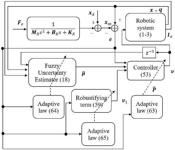
The Block diagram of the control system
The dynamic equation of electrically driven robot manipulators in task-space can be obtained by substituting equation (1) to (2) and using equations (4), and (5) and (9) as follows
Some properties of the dynamic equation of electrically driven robot manipulators (Eq. 27) can be expressed as follows [26]:
Property 1:
The matrix Dx is a symmetric positive definite matrix for all x ∈ Rm.
Property 2:
The skew-symmetric properties is preserved for
Property 3:
The task-space dynamic equation can also be linearly parameterized with using a suitable selected parameter vector
Let us define the error dynamics as
Consider a following positive definite function as
Taking the time derivative of V gives that
Using (33) and (34), equation (36) yields
One can rewrite equation (27) as
Substituting (39) into (38) we have
Considering (33) and (34), one can obtain
Thus, substituting (41) into (40) yields to
In other words,
Let us define the modified velocity and acceleration in task-space as follows
By using the skew-symmetric property (31) and equations (44) and (45), one can modify (43) as
Considering linear parameterization property (32), we can write
It is noted that
Remark 4.
Researchers have faced difficulties in analyzing the motion equation in task-space since the exact kinematics model is not available in practice or surplus of sensors is required to monitor the motion of an end-effector. To deal this problem, let us consider the transformation functions as follows
By applying (49) and (50) to equation (47) and using (28–30), it can be obtained
Using (51) and also transforming the error dynamics (33) into joint space, i.e.
This paper proposes the control law as
Assume that
Using the Cauchy–Schwartz inequality, we have
The robustifying term is selected as
By substituting (59) in (58) and some manipulations, we have
Assume that the uncertainty (10) can be modelled as
If the adaptation laws are chosen as
Then equation (62) is expressed as
The following assumptions are made to complete the stability analysis [26,30]:
Assumption 1
The desired trajectory xd must be smooth in the sense that xd and its derivatives up to a necessary order are available and all uniformly bounded.
Assumption 2
The external disturbance φ(t) is bounded as ‖φ(t)‖ ≤ φmax.
where φmax is the maximum value for the external disturbance. The electric motors should be protected against over-voltage, thus the next assumption is considered.
Assumption 3
The motor voltage is bounded as ‖v(t)‖ ≤ vmax.
The error dynamics,
Since k2 is a positive definite matrix, then the right-hand side of (67) is bounded as
Using the Cauchy–Schwartz inequality and considering the upper bound of modelling error as ‖εf‖ < ρ, the left-hand side of (67) can be obtained
Therefore, by considering (68) and (69) in order to satisfy
In other words
Let us define two diagonal positive definite matrices k21 and k22 such that k2 = k21 + k22 (i.e. λmin(k2) = λmin(k21) + λmin(k22)), in order to satisfy
As a result, in order to satisfy (67), it is sufficient that
Considering assumption 2 and 3 and the proof given by [31], v, Ia,
6. Simulation results
The proposed control approach is applied for the robust control of the electrically driven two-link elbow manipulator. The dynamic parameters of the robot and the motors’ parameters have been presented in Table. 1 and Table 2, respectively. The desired position trajectory for end-effector, as illustrated in Fig. 2, is formulated by
| Parameters | Value |
|---|---|
| l1, l2 (m) | 1 |
| lc1, lc2 (m) | 0.5 |
| m1 (kg) | 15 |
| m2 (kg) | 6 |
| I1 (kg. m2) | 5 |
| I2 (kg. m2) | 2 |
Dynamic parameters of two-link planar arm
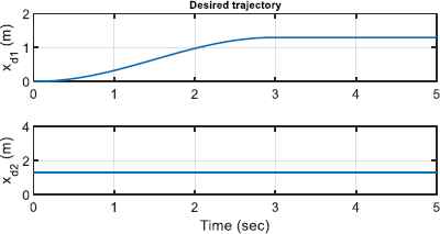
Desired Trajectory
| Parameters | Value |
|---|---|
| umax(V) | 40 |
| R (Ω) | 1.6 |
| L (H) | 0.001 |
| Kb (V. s/rad) | 0.26 |
| Km (N. m/A) | 0.26 |
| Jm (Nm. s2/rad) | 0.0002 |
| Bm (Nm. s/rad) | 0.001 |
| r | 0.02 |
The specifications of permanent magnet dc motors.
Remark 5.
To perform simulation and according to Remark 4, one can use inverse kinematics in order to obtain the joint variables in terms of the x and y coordinates. Considering Fig. 3 and using the Law of cosines, we have
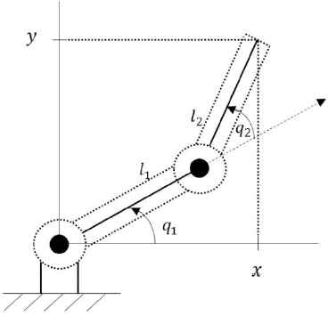
A two-link planar arm
Simulation 1. The environment model with xe = [1.29 y]T m and Ke = diag(100000,0) N ⁄ m is given by
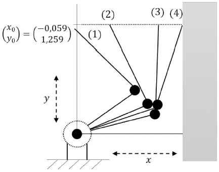
Schematic plot of robotic trajectory
The contact force between the end-effector and environment is depicted in Fig .5. As shown, the contact phenomenon occurs in 2.84 sec and the generated force reaches rapidly a maximum value of 122.1 N. From this time forward, the proposed compensator comes into operation and efficiently compensates the harmful effect of the contact and finally makes the contact force approximately decrease to 4 N.
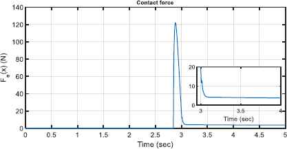
The contact force between the end-effector and environment
Motors behave well under the permitted voltages as shown in Fig. 6. The interaction effect of end-effector and environment for both motors’ voltages at t = 2.84 sec is detectable. Also, it is noted that from the contact between the end-effector and environment forward, both motors approximately tolerate constant voltages. Fig. 7 illustrates the performance of control approach providing similar behavior of robotic system and the reference model such that the reference errors are reduced well to the range of [–2.5 2.5] × 10−3 m. The tracking performance of the reference model is shown in Fig 8. The first reference model tracking error, i.e. xd1 − xm1, shows that the contact between the end effector and the environment occurs at t = 2.84 sec along the x axis. The second signal of reference model, xm2, does not show any deviation from the desired signal, xd2, since there is no force along the y axis. It is noted that by increasing the first model reference tracking error, the control approach protects the robot and the environment from the possible detrimental effect of the contact. To do this, according to Figure (5) and Figure (8), the contact force finally decreases to 4 N such that the second signal of reference model for the end-effector is deviated approximately 9mm along the x axis. Figure. 9 shows the adaptive fuzzy parameters (Eq. 64),
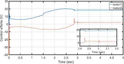
Control efforts of the proposed control approach
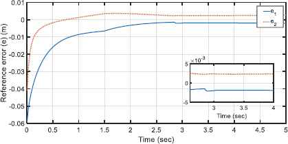
The reference errors (Eq. 34)
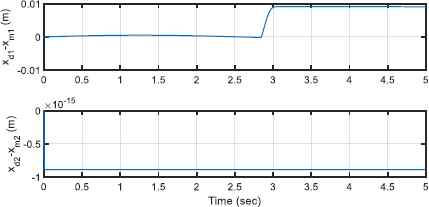
Tracking performance of the reference model
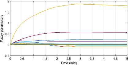
Adaptation of uncertainty fuzzy parameters
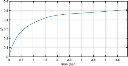
Adaptation of parameter
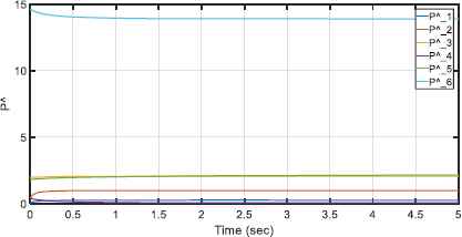
Adaptation of
Simulation 2. The performance of the proposed controller is evaluated by different stiffness of the environments. To perform simulation, four values for Ke are chosen as Ke1 = diag(20000,0), Ke2 = diag(60000,0), Ke3 = diag(100000,0) and Ke4 = diag(140000,0). Fig. 12 and Fig. 13 illustrate the contact force between the end-effector and different environments and the performance of the control method interacting with environments with different stiffness, respectively.
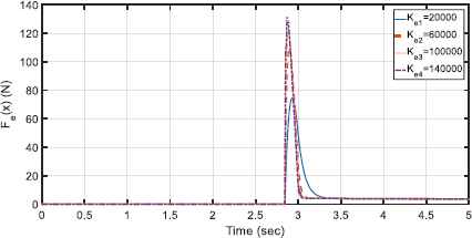
The contact force between the end-effector and environments with different stiffness
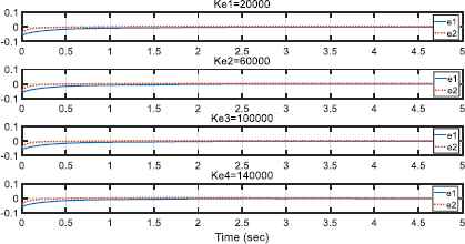
The performance of the control method interacting with environments with different stiffness
7. Conclusion
This paper has proposed a model-reference impedance control approach using fuzzy uncertainty estimator for the robust control of electrically driven robot manipulators. In the proposed control method, a desired dynamical behavior of the robot interacting with an environment is considered as the model-reference such that this model-reference provides a reference signal for a robot whether in tracking or contact situations. As the interaction between an end-effector and an environment occurs, the contact force is exerted to the model-reference and the robotic system receives the output of model-reference as a desired trajectory and thus the aim of the controller is to reduce the difference between the task space desired trajectory and the desired impedance model. It is worth noting that the feedback of contact force is not utilized in the structure of the proposed controller and the adaptive laws since by increasing the contact force at the time of the interaction between an end-effector and an environment, existing the contact force will cause problematic issues for control designers. Furthermore, to improve the performance of control system and also compensate un-modelled dynamics and external disturbances, two control terms namely a robustifying term and a fuzzy uncertainty estimator are employed in the structure of the controller. The proposed control approach has shown a good performance in terms of simplicity in design, high-performance of contact force compensation and small reference error. The stability analysis has been guaranteed by the proposed control method and the simulation results verified the effectiveness of the method.
Appendix A.
The regressor matrix
References:
Cite this article
TY  - JOUR
AU  - Gholamreza Nazmara
AU  - Mohammad Mehdi Fateh
AU  - Seyed Mohammad Ahmadi
PY  - 2018
DA  - 2018/05/03
TI  - A model-reference impedance control of robot manipulators using an adaptive fuzzy uncertainty estimator
JO  - International Journal of Computational Intelligence Systems
SP  - 979
EP  - 990
VL  - 11
IS  - 1
SN  - 1875-6883
UR  - https://doi.org/10.2991/ijcis.11.1.74
DO  - 10.2991/ijcis.11.1.74
ID  - Nazmara2018
ER  -