
Tire Defects Classification Using Convolution Architecture for Fast Feature Embedding
Equal Contributors
- DOI
- 10.2991/ijcis.11.1.80How to use a DOI?
- Keywords
- Deep learning; Defect classification; CNN; AlexNet; Tire defects
- Abstract
Convolutional Neural Network (CNN) has become an increasingly important research field in machine learning and computer vision. Deep image features can be learned and subsequently used for detection, classification and retrieval tasks in an end-to-end model. In this paper, a supervised feature embedded deep learning based tire defects classification method is proposed. We probe into deep learning based image classification problems with application to real-world industrial tasks. Combined regularization techniques are applied for training to boost the performance. Experimental results show that our scheme receives satisfactory classification accuracy and outperforms state-of-the-art methods.
- Copyright
- © 2018, the Authors. Published by Atlantis Press.
- Open Access
- This is an open access article under the CC BY-NC license (http://creativecommons.org/licences/by-nc/4.0/).
1. Introduction
There has been an increasing interest in the use of NDT techniques of defects from steel [1], castings [2], [3], textile [4], TFT-LCD panel [5], nanostructures [6], [7], titanium-coated aluminum surfaces [8], and semiconductors [9] etc. Among these topics, tire defects inspection research is a significant research topic that has been investigated by researchers from both academy and industry areas over the past few decades [10], [11], [12], [13], [14] and is considered as one of the most challenging problems in industrial information revolution era [15] due to its unique properties illustrated in our previous study [11]. Much work has been done on automatic tire defect detection and has been applied in tire X-ray inspection systems to carry out computer vision based automatic defect inspection. Tire defect classification is one of the three steps in computer vision (radiographic) based tire inspection in which the first step is an X-ray imaging system, the second is defect detection and the last one is defect classification. However, in most real-world applications tire defect classification and defective products handling thereafter still require human observers. The reason for this is that the complexity, high-variety, and high dynamic range real-world defect pattern cannot be described with analytical equations. Because the dynamics are either too complex or unknown and traditional shallow methods, which contain only a small number of non-linear operations, do not have the capacity to accurately model such complex data [16]. In previous work, low-level features were used for tire defects detection and classification. In [11], optimal scale and threshold parameters were selected to distinguish defect edges from the background textures using wavelet multi-scale features. To model complex real-world data, exquisite features, either supervised or semi-supervised, are selected to capture relevant information in classification tasks.
However, on the one hand, developing domain-specific features for each specific task is expensive, time-consuming, and requires expertise of the data. On the other hand, unsupervised feature learning [17], [18] is an alternative to learn feature representations from unlabeled data which would result in performance degeneration because of overfiting when a large number of features are utilized. Dimensionality reduction and feature selection techniques have been applied to address the problem of dimensionality, which is becoming a significant branch in the machine learning and data mining research area [19], [20].
Deep networks, with the goal of learning to produce a useful higher-level representation from the lower-level representation output by the previous layer from unlabeled data, are motivated in part by knowledge of the layered architecture of regions of the human brain such as the visual cortex, and in part by a body of theoretical arguments in its favor [21]. Deep networks have been used to achieve state-of-the-art results on a number of benchmark datasets for solving difficult artificial intelligence (AI) tasks. A variety of deep learning algorithms have been proposed, e.g., Deep sparse auto encoders (Bengio) [22], Stack sparse coding algorithm [23], Deep Belief Network (DBN) (Hinton) [24] and their extrapolations, which learn rich feature hierarchies from unlabeled data and can capture complex invariance in visual patterns. In recent ImageNet Large Scale Visual Recognition Challenge (ILSVRC) competitions [25], deep learning methods have shown to be successful for computer vision tasks by extracting appropriate features while jointly performing discrimination and thus have been widely adopted by different researchers and achieved top accuracy scores [26], [27]. There have been applications based on these techniques in diverse vision tasks. In [28], Shi and Zhou et al. proposed a stacked deep polynomial network based representation learning method for tumor classification. A discriminant deep belief network was proposed in [29] to characterize SAR image patches in an unsupervised manner in which weak decision spaces were constructed based on the learned prototypes. Various deep learning approaches have been extensively reviewed and discussed in [27].
However, much work has been done in the deep learning community, researchers focus mainly on developing models for static data and not so much on optimal representation for practitioners in real-world applications, e.g., what makes a optimal representation for practitioners in real-world applications; and can unsupervised pre-training criteria be applied to initialize deep networks for better classification?
In this work, a supervised feature embedded deep learning based tire defect classification method is proposed. We probe into deep learning based image classification problems with application to real-world industrial tasks. The deployment of deep neural networks in industrial application domains are well explored and discussed.
This paper is organized as follows. Section 2 provides an overview of deep learning model and architecture. Starting from the related work of CNN based deep feature learning and Caffe (Convolution Architecture for Feature Embedding, Caffe) framework, we discuss related existing works and present a generalized formulation of the state-of-the-art AlexNet architecture. In section 3, we describe the dataset used in this work and introduce data preparation and augmentation processes. Section 4 presents experiments that qualitatively study of classification accuracies for each tire defect category and validates the effectiveness of the scheme compared with other state-of-the-art methods using the same dataset. Section 5 summarizes our findings and concludes our work.
2. Deep Network Model for Learning Representations
Different from the general idea of face recognition, universal object recognition, which aims at learning thousands of objects from millions of images, is becoming a booming research field while still is a huge challenge for the reason that datasets contain a huge number of features, noise, and a variety scale of different objects which exceeds the capacity of traditional classification schemes. The problem to be addressed in this work however, faces similar difficulties such as multiple categories, scale varieties, magnanimous features and noise.
To describe object instances, various local features such as Scale Invariant Feature Transform (SIFT) [30] and its variants like Speeded-Up Robust Features (SURF) [31] etc., binary descriptors including FREAK [32] and BRISK [33], are extracted, with or without embedding them into Global Features Representations. For example, BRISK is a 512-bit binary descriptor that computes the weighted Gaussian average over a select pattern of points near the key point. However, in some real-world applications, existing classification methods using a Bag of Words model based on low level features and global representations as well cannot yield satisfactory presentations, especially when the high-level concepts in the user’s mind is not easily expressible in terms of the low-level features as is shown in Fig. 1.
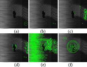
Low level features of tire radiography image. (a) Brisk; (b) FAST; (c) Harris; (d) MinEigen; (e) MSER; and (f) SURF.
In recent years, by virtue of its appropriate features representation and their jointly discrimination, deep networks have been shown to be successful for computer vision tasks [34], [35] and have outstripped traditional techniques in the ILSVRC (ImageNet Large Scale Visual Recognition Challenge, ILSVRC) which has become the standard benchmark for large-scale object detection as well as image classification since 2010. In 2012, as the major milestone of deep learning based methods AlexNet [36] trained on ImageNet 2012 reached a great success in the ILSVRC after which deep learning based methods such as ZF [37], SPP [38] and VGG [39] choose AlexNet as their baseline deep model and also achieved excellent performance. Thereafter more approaches [38], [40], [41] were proposed based on the scheme by fine-tuning the parameters according to their specific applications. However, few toolboxes or trained models of published results offer truly off-the-shelf deployment of state-of-the-art models such that they are not sufficient for real-world applications or even commercial deployment.
To address such problems, a fully open-source framework Caffe was proposed to afford clear access to deep architectures [42]. Caffe is an open-source deep learning framework for state-of-the-art deep learning algorithms and a collection of reference models. The framework provides a complete toolkit for training, testing, fine tuning, and deploying models. Moreover, it is one of the fastest available implementation of these algorithms, making it immediately useful for industrial deployment. In this work, we address the tire defects classification using deep learning based on convolution neural network under the Caffe framework.
Compared with previous schemes such as Cifar 10 and LeNet, AlexNet has been improved by Hinton et al. by adding Rectified Linear Units (ReLU) nonlinearity and Dropout [43] model regularization strategy at fully-connected layers which make it several times faster than their equivalents and prevent substantial overfitting at the same time. Fig. 2 shows the flowchart of the proposed tire defects classification scheme.
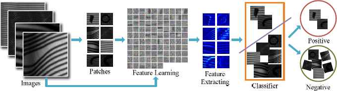
The flowchart of the proposed tire defects classification scheme.
2.1. Network architecture
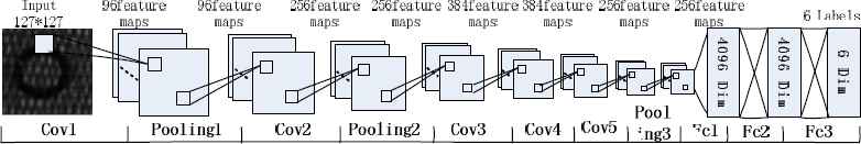
As a milestone of CNN based deep learning scheme, AlexNet has a significant architecture. As is shown in Fig. 3, in this work there are five convolutional layers namely conv1, conv2, conv3, conv4 and conv5 with kernel sizes 11×11, 5×5, 3 × 3, 3 × 3 and 3 × 3 pixels respectively. Considering the geometric dimensions and scales of tire defects in the dataset, we set the fixed-resolution (127 × 127) images as the input to the first convolutional layer which with 96 kernels of size 11 × 11with a stride of 4 pixels. The second convolutional layer filters the output of pooled output of the first convolutional layer with 256 kernels of size 5 × 5 and with a stride of 1 pixel. The pooled output of the second convolutional layer is connected to the rest three convolutional layers without using any pooling layers with 384, 384 and 256 kernels of size 3 × 3 and with a stride of 1 pixel respectively. The fifth convolutional layer is followed by a max-pooling layer and two fully-connected layers which have 4096 neurons each. Finally, the output of the last fully-connected layer is fed to soft max which produces a distribution over the 6 class labels as is shown in Fig. 3.
The flowchart of the proposed tire defects classification scheme.
In this architecture, three max-pooling layers are used after the first, second and fifth convolutional layers with the pooling size of 32 pixels and the stride of 2 pixels. In each fully-connected layer, ReLU non-linearity activation function is applied for a better convergence speed than that using sigmoid and tanh activation functions. A more detailed configurations and primary parameters of the CNN model are listed in Table I.
| Layer | Type | Maps & neurons | Kernel | Stride |
|---|---|---|---|---|
| 0 | Input | 3 maps of 127×127 neurons | ||
| 1 | Convolutional | 96 maps of 30×30 neurons | 11×11 | 4 |
| 2 | Max pooling | 96 maps of 15×15 neurons | 3×3 | 2 |
| 3 | Convolutional | 256 maps of 15×15 neurons | 5×5 | 1 |
| 4 | Max pooling | 256 maps of 7×7 neurons | 3×3 | 2 |
| 5 | Convolutional | 384 maps of 7×7 neurons | 3×3 | 1 |
| 6 | Convolutional | 384 maps of 7×7 neurons | 3×3 | 1 |
| 7 | Convolutional | 256 maps of 7×7 neurons | 3×3 | 1 |
| 8 | Max pooling | 256 maps of 3×3 neurons | 3×3 | 2 |
| 9 | Fully connected | 4096 neurons | 1×1 | 1 |
| 10 | Fully connected | 4096 neurons | 1×1 | 1 |
| 11 | Fully connected | 6 neurons | 1×1 | 1 |
Network architecture.
2.2. Pre-training and fine-tuning
Consider that our dataset has limited quantities of samples, in this work we used a pre-trained network on ImageNet to initialize the networks with pre-trained parameters and thus to accelerate the learning process and to improve the generalization ability. Moreover, data augmentation and dropout techniques were used to regulate data.
There are many research works indicated the feasibility and efficiency of transferring the pre-trained model to new tasks with a variety of datasets [44]. They indicated how well features at that layer transfers from one task to another and concluded that initializing a network with transferred features from almost any number of layers can give a boost to generalization performance after fine-tuning to a new dataset. To adapt the pre-trained nets to our specific classification task, fine-tuning process is necessarily of great concern. We use the pre-trained AlexNet model to initialize all layers except the output layer in which a limited number of category labels are used compared with that in the ILSVRC.
Class labels are given for our new training dataset to compute the loss functions. Moreover, in this work, we decrease the spatial resolution of each hidden layer, and thus to increase the number of feature plane in order to detect more types of features for tire defects. A more detailed network architecture that illustrates the fine-tuning process will be given in Section 4.
The most direct way to improve the feature representation or classification ability of CNNs is to use a deeper network and more neurons, namely deeper and wider. However, deeper networks also bring over-fitting problem. Existing studies have shown that dropout technique helps preventing overfitting even though this roughly doubles the number of iterations required to converge. Because the neurons which are “dropped out” do not contributed to the forward pass and do not participate in backpropagation. A neuron cannot rely on the presence of particular other neurons. In this work, we use dropout in the first two fully-connected layers with dropout_ratio=0.5 as is shown in Fig. 3.
3. Dataset
3.1. Data Source
In this work, a dataset composed of 1582 images belonging to 6 typical defect categories, namely Belt-Foreign-Matter (BFM), Sidewall-Foreign-Matter (SFM), Belt-Joint-Open (BJO), Cords-Distance (CD), Bulk-Sidewall (BS) and Normal-Cords (NC), was used to perform the tire defect classification experiments. The images were collected from a typical tire manufacturing enterprise in China. Source images were derived from real-world defect detection system at the end of the manufacturing line and thereafter were labeled manually by human labelers. Moreover, the proportion of defect samples is consistent with that of the production line. Fig. 4 shows sample synopses of the evolving dataset.
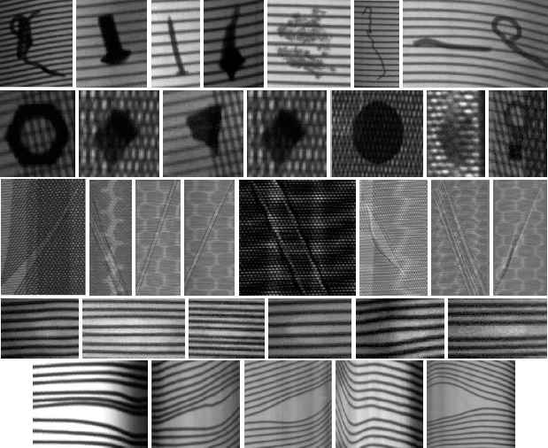
Sample synopses of the evolving dataset (Some of the images above were scaled for better visual effect). From top to bottom: Sidewall-Foreign-Matter, Belt-Foreign-Matter, Belt-Joint-Open, Bulk-Sidewall, Cords-Distance.
3.2. Data Preparation and Augmentation
According to the statistics on the tire defects dataset, it consists of variable-resolution defect images arrange between 50×50 and 200×500 pixels due to the uncertainty of tire defects occurrences in the production. In order to meet the requirements of a constant input dimensionality of the classification scheme, characterize tire defects to the maximum extent and reduce computational complexity at the same time, the images in the dataset were down-sampled or up-sampled to a fixed resolution of 127×127. Given a rectangular image, we first rescaled the image such that the shorter side was of length 127, and then cropped out the central 127×127 patch from the resulting image. We did not pre-process the images in any other way, except for subtracting the mean activity over the training set from each pixel. Therefore, aiming at practical applications, raw gray values of the pixels are used in this work.
In deep learning based tasks, sufficient amount of data is usually needed to avoid severe overfitting problem. Under different applications, the geometric transformation of the image using one or more combination of data augmentation transform can be used to increase the amount of input data. In AlexNet, two forms of data augmentation were employed: image translations and horizontal reflections and altering the intensities of the RGB channels while in Fast R-CNN [45] only horizontal flip was used. In this work, we abandon altering the intensities of the RGB channels given that the radiographic images are in gray value in our dataset and add reflection, zoom, scale and contrast translations to produce more training examples with broad coverage.
4. Experiments and Discussion
The performance of the proposed deep learning scheme was evaluated by applying it to our tire defects dataset. For test, 20% of each defect category were selected randomly as test dataset, another 20% of each defect category are selected randomly as validation dataset, and the rest were selected as training dataset. Ten groups of selections were used for experiments and their mean classification accuracy was taken as the final results.
We use images with fixed resolution of 127×127 as the input of the network which would convolve and pool the activations repeatedly, then forward the results into the fully-connected layers and classify the data stream into 6 categories. Considering the small quantities of validation dataset, to prevent the error descending too fast we set the initial learning rate base-lr as 0.001. For test dataset, we set test batch volume batch as 246, test batch test-iter as 1, and test interval test-interval=200, namely test once every 200 iterations and displays classification accuracy. Unlike AlexNet in which two GPUs are used, in this work we set the solver_mode as CPU. The remaining parameters of the deep architecture were the same as the default parameters in the CaffeNet optimization model.
Fig. 5 shows the filters on the first convolutional layer (upper left), and the second convolutional layer (upper right) of the network and filtered features respectively. Notice that the weights of the first convolutional layer are smooth and without noisy patterns, indicating nicely converged network while the second convolutional layer weights are not as interpretable, but it is apparent that they are still smooth, well-formed which would guarantee high regularization strength to avoid overfitting.
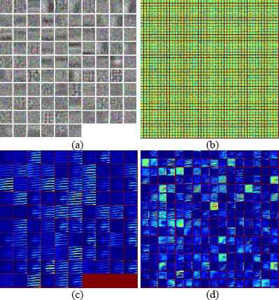
(a) Filters on the first convolutional layer, and (b) the second convolutional layer of the network, (c) and (d) filtered features respectively.
In the three fully-connected layers, Fc6 and Fc7 are hidden layers with 4096 neurons while Fc8 is the soft max output layer of 6 categories. Fig. 6 (upper row) shows the statistics of Fc6 and Fc7 in which the horizontal axis represents the number of neurons and the vertical axis represents each neuron's response value. Fig. 6 (bottom row) shows the histogram respectively, the horizontal axis is the neuronal response value, the vertical axis is the number of occurrences of each response value.
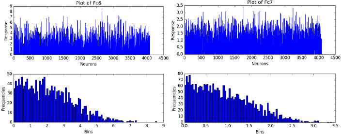
The statistics of fully-connected layers (Fc) Fc6 and Fc7.
Fig. 7 illustrates the classification accuracy versus loss relation graph in which the horizontal axis denotes the number of iterations while the left vertical axis representing the value of the loss function (LF) and the right vertical axis denotes the average validation recognition rate. The loss function represents the price paid for inaccuracy of predictions in classification and therefore measures the optimal strategy. The smaller the LF value is the better the system is. As can be seen in Fig. 5, after 1200 iterations the loss curve tends to zero while the classification accuracy curve tends to 1 which meet the requirements of the optimization objectives. The validation classification accurate reaches as high as 0.98374 when the iteration is 1200 while decreases to 0.97561 when the iteration is 2000 and, the actual test accuracy is 0.94521.
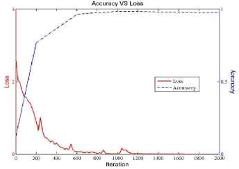
The relation between classification accuracy and the loss function value.
Table II shows the detailed classification accuracies for each tire defect category. As is shown that the overall classification accuracy reaches 96.51% for all categories. Correct classification accuracy for BS defect is the lowest, 88.89%, while SFM and BFM defects own the highest correct classification accuracies, 100%, among all categories. BS defects were mainly mistakenly classified as normal cords which is because the weak edge of tire BS defect is too weak to be extracted by the feature representation scheme. Most of BS defects can't be identified even by qualified human observers as is shown in Table II.
| Positive/Negtive classification | SFM | BFM | BJO | CD | BS | NC | Correct classification | Total sample | Accuracy % |
|---|---|---|---|---|---|---|---|---|---|
| SFM | 68 | 0 | 0 | 0 | 0 | 0 | 68 | 68 | 100 |
| BFM | 0 | 53 | 0 | 0 | 0 | 0 | 53 | 53 | 100 |
| BJO | 0 | 2 | 50 | 0 | 0 | 0 | 50 | 52 | 96.15 |
| CD | 0 | 0 | 0 | 53 | 1 | 1 | 53 | 55 | 96.36 |
| BS | 0 | 0 | 0 | 0 | 40 | 5 | 40 | 45 | 88.89 |
| NC | 0 | 0 | 0 | 0 | 2 | 41 | 41 | 43 | 95.35 |
| Total sample | 305 | 316 | 96.51 |
Detailed classification accuracies for each tire defect categories.
On the other hand, the scheme reached satisfactory classification accuracies for other tire defect categories, especially for SFM and BFM defects, 100% accuracies were reached. Deep learning is almost the only end-to-end machine learning system available in which the most expressive deep features can be learnt and classified automatically. This mechanism therefore is consistent with the human visual process.
To validate the effectiveness of the scheme, we experimented on available state-of-the-art methods for a general comparison on the same dataset, shown in Table III. We experimented PCA+BP neural network, ScSPM09 [46], LLC10 [47], KSPM-200-3 [48], KSPM-400-2 [48] and LeNet [49] methods. Here in KSPM-200-3 method, we set dictionary size N=200 with a 3 layer pyramids structure while in KSPM-400-2 we set N=400 with pyramid structure of 2 layers. SIFT features were used in ScSPM09, LLC10 and KSPM methods, and linear SVM classifier was used in ScSPM09 and LLC10 methods while in KSPM-200-3 and KSPM-400-2 methods nonlinear SVM classifier was used. As is shown in Table III that our method outperformed state-of-the-art methods on our tire defect dataset with the overall classification accuracy of 96.51% and validation classification accuracy of 98.37%.
| Methods | Overall Accuracy % |
Validation Accuracy % |
Test times In second |
|---|---|---|---|
| PCA+BP | 69.44 | / | 30.23 |
| ScSPM09 | 95.56 | / | 84.67 |
| LLC10 | 94.85 | / | 22.37 |
| KSPM-200-3 | 92.77 | / | 15.26 |
| KSPM-400-2 | 92.37 | / | 15.35 |
| LeNet | 91.89 | 93.46 | 26.36 |
| Our method | 96.51 | 98.37 | 37.16 |
Comparison on state-of-the-art methods using the same dataset.
Notice that the validation classification accuracies are slightly better than the test overall classification accuracies in both LeNet and our method. There are two reasons for this. Firstly, insufficient training samples were used. And secondly, parameters were not optimized. Given that tires are of nonlinear composite material structure, the manufacturing process is complicated such that there are a broad variety of tire defects with different shapes, scales, positions and gray levels etc. that consist of large number of features in both foreground and background of radiographic images. On the other hand, deep nets have a too large number of parameters to be trained that only large quantities of training samples can be sufficient for training a network with strong generalization capability. ScSPM09 and LLC10 are two successful sparse coding based methods that have been extensively studied and applied in various domains. Both of them received acceptable classification accuracies however, in the two methods and KSPM method researchers need to be involved in the extraction of image features and the selection of classifiers. Most importantly, these selections would affect the classification accuracies directly.
Compared with these methods, the proposed scheme outperformed them in classification by virtue of the advantages of CNNs such as well-matched topology structure of the input image and the network, weight sharing and feature representation etc. However, it is worth noting that the relationship between network’s size and performance can be complicated even though it is believed that with a larger network the results can be improved under this deep convolutional neural network architecture.
The last 3 layers of the given model are fully connected layers (Fc6~Fc8). Notice also that prior convolution and the pooling layers have reduced the dimensionality of the features to the acceptable size such that the use of the three fully connected layers will not result in a serious computational burden. The test time of the proposed method for the test dataset is 37.16s on a workstation with 3.60 GHz 4-core CPUs and 16 GB RAM, on an Ubuntu 16.04, Caffe and python 2.7 platform. The average processing time of the proposed method for the final representation of an input image is 0.1176 seconds. The LetNet method was tested on the same platform and workstation. The PCA+BP, ScSPM09, LLC10 and KSPM methods were tested in MATLAB R2009b, on a 64-bit Windows 7 platform, on the same workstation. A detailed test times comparison is shown in Table III.
5. Conclusions
In just a few years, deep learning almost subverts the thinking of image classification, speech recognition and many other fields, and are forming an end-to-end model in which the most reprehensive deep features can be learnt and classified automatically. This model tends to make everything easier. Moreover, in deep nets each layer can be adjusted according to the final task and ultimately to achieve co-operation between the layers which can greatly improve the accuracy of the task. However, the detection and classification of universal objects or generalized automatic deployment, e.g. tire defects, is often an ambiguous and challenging task especially in real-world application. Inspired by recent successful approaches, the approach we investigate in the present work, that is, using a supervised feature embedded deep learning based scheme to classify tire defects which is an application of deep learning to real-world industrial tasks. Combined regularization techniques were applied for training to boost the performance. Experimental results show that our scheme received satisfactory classification accuracy and outperform state-of-the-art methods. This work would provide practical usefulness to both researchers and practitioners in various industrial fields.
Acknowledgements
This work was supported by the National Natural Science Foundation of China No. 61472196, by the Shandong Provincial Natural Science Foundation under Grant No. ZR2014FL021, by the Applied Basic Research Project of Qingdao Grant No. 15-9-1-83-JCH and by the Doctoral Found of QUST under Grant No. 010022671.
6. References
Cite this article
TY  - JOUR
AU  - Yan Zhang
AU  - Xuehong Cui
AU  - Yun Liu
AU  - Bin Yu
PY  - 2018
DA  - 2018/05/23
TI  - Tire Defects Classification Using Convolution Architecture for Fast Feature Embedding
JO  - International Journal of Computational Intelligence Systems
SP  - 1056
EP  - 1066
VL  - 11
IS  - 1
SN  - 1875-6883
UR  - https://doi.org/10.2991/ijcis.11.1.80
DO  - 10.2991/ijcis.11.1.80
ID  - Zhang2018
ER  -