
Interval-valued Pythagorean Fuzzy Frank Power Aggregation Operators based on An Isomorphic Frank Dual Triple
- DOI
- 10.2991/ijcis.11.1.83How to use a DOI?
- Keywords
- Interval-valued Pythagorean fuzzy numbers; Frank dual triple; Frank power operators
- Abstract
Interval-valued Pythagorean fuzzy sets (PFSs), as an extension of PFSs, have strong potential in the management of complex uncertainty in real-world applications. This study aims to develop several interval-valued Pythagorean fuzzy Frank power (IVPFFP) aggregation operators with an adjustable parameter via the integration of an isomorphic Frank dual triple. First, a special automorphism on unit interval is introduced to construct an isomorphic Frank dual triple; and this triple is further applied on the definition of interval-valued Pythagorean fuzzy Frank operational laws. Second, two IVPFFP aggregation operators with the inclusion of an adjustable parameter are defined on the basis of the proposed operational laws, and several instrumental properties are then investigated. Furthermore, some limiting cases of the proposed IVPFFP operators are analyzed with respect to the varying adjustable parameter values. Finally, an IVPFFP aggregation operator-based multiple attribute group decision-making model is developed with a practical example furnished to demonstrate its feasibility and efficiency. The power that the adjustable parameter exhibits has been leveraged to affect the final decision results, and the proposed IVPFFP operators are compared with three selected aggregation operators to demonstrate their advantages provided with a practical example.
- Copyright
- © 2018 Yang et al.
- Open Access
- This is an open access article under the CC BY-NC license (http://creativecommons.org/licences/by-nc/4.0/).
1. Introduction
The term Pythagorean fuzzy set (PFS)1,2 was coined by Yager as a powerful extension of intuitionistic fuzzy set (IFS)3. PFS, akin to IFS, is composed of membership grade μ and nonmembership grade v and is further delivered to form a binary group representation. The core distinction between IFS and PFS is reflected in the constraint of the grade pairs, which is μ + v ⩽ 1 for IFS and is μ2 + v2 ⩽ 1 for PFS. PFSs include IFSs as a whole and pose few barriers of information representation. A plethora of practical applications of PFS have demonstrated its utility in addressing multiple attribute group decision-making (MAGDM) problems4–9,36. The main characteristic of the membership and nonmembership degrees of PFS is that their values are often expressed as real numbers. However, in certain cases, decision makers (DMs) may only be able to provide a range of values for these grades. Consequently, PFS is not applicable to these cases. In view of this deficiency, the notion of interval-valued PFS (IVPFS) was further developed10,11. IVPFS enables DMs to express their uncertainty via the provision of interval-valued membership and nonmembership values. Several researchers have conducted related studies on the application of IVPFS in MAGDM10–13.
In developing various fuzzy sets such as IFS, hesitant fuzzy set (HFS) and hesitant-intuitionistic (or dual hesitant) fuzzy set, the basic operations for them play an indispensable role, which is also not an exception for IVPFS. However, few studies on the operations for IVPFS have been conducted10,11, especially the generalized operations. In fact, some generalized operations on various types of extended fuzzy sets have been developed on the basis of the Frank dual triple, such as intuitionistic Frank operations14,15, interval-valued intuitionistic Frank operations16, hesitant Frank operations17, triangular interval type-2 fuzzy Frank operations18, interval intuitionistic linguistic Frank operations19 and dual hesitant fuzzy Frank operations20. The Frank dual triple consists of a standard negation, Frank t-norm, and its dual s-norm21 with the adjustable parameter χ. A desirable feature of this triple is that DMs can select different values to obtain various types of dual triple. In the cases of χ → 1 and χ → ∞, for example, then Frank dual triple will reduce to the algebraic dual triple and the Lukasiewicz dual triple, respectively. However, a numerical example will be provided to reveal that the Frank dual triple is not suitable for defining the generalized operations on IVPFSs. In view of the reasons mentioned before, an automorphism on [0,1] will be introduced in this study to develop an isomorphic Frank dual triple, which includes an isomorphic Frank t-norm, an isomorphic Frank s-norm and the Pythagorean negation1,2. Then, this new dual triple can be used to define the Frank operations on IVPFSs.
A core step of MAGDM is to aggregate multiple assessment matrixes into a synthesis assessment matrix, which is often performed by appropriately selecting aggregation operators31,32. Recently, some aggregation operators have been proposed to fuse multiple interval-valued Pythagorean fuzzy numbers (IVPFNs), such as IVPFWA and IVPFWG aggregation operators10,12,13. To deal with the correlation among the input arguments in MAGDM problems, many studies22–25 have used power average (PA) to successfully model such situation26. Thus, in this study, the PA and power geometric (PG) operators27 were extended to IVPFSs. Inspired by their research, the Frank operational laws will be used to propose the interval-valued Pythagorean fuzzy Frank power weighted average (IVPFFPWA) and interval-valued Pythagorean fuzzy Frank power weighted geometric (IVPFFPWG) aggregation operators. A prominent feature of the aggregation weights for the two aggregation operators is that they not only consider the importance of experts but also depend upon the supports from the remaining input IVPFNs. Moreover, the relationships between the Pythagorean Frank aggregation operators and their related adjustable parameters will be analyzed, and some limiting cases of these operators will as well be investigated. Finally, by applying the proposed Frank aggregation operators, a novel decision making approach is constructed to deal with the MAGDM problem with IVPFNs. With the numerical example provided, the relationship between the proposed aggregation operators and their adjustable parameters can be explained accordingly.
The rest of paper is structured as follows. Relevant definitions of IVPFSs are reviewed in Section 2. Section 3 proposes an isomorphic Frank dual triple, which is then used to define the Frank operations for IVPFSs. Subsequently, the IVPFFPWA and IVPFFPWG aggregation operators are developed in Section 4. Section 5 applies the proposed aggregation operators to develop a simple decision-making approach to solving MAGDM with IVPFNs. An illustrative example is provided to verify the proposed approach in Section 6. Finally, section 7 concludes this paper.
2. Preliminaries
Relevant definitions of IVPFSs are reviewed and the dual triple, which consists of t-norm, s-norm, and negation, is introduced along with its components. Particular attention will be paid to the Frank dual triple. We then provide the definition of isomorphism dual triple, which is essential in this study.
2.1. Related definitions of IVPFSs
Definition 1. 3
Let K denote a finite universal set, and then a IFS B on K is provided as
Definition 2. 1,2
Given a finite universal set K, a PFS P on K is defined as
Definition 3. 10,11
Given a finite universal set K, and IVPFS
Definition 4. 10,11
Let
- (1)
- (2)
Definition 5. 10,11.
Let
- (1)
- (2)
- (3)
- (4)
- (5)
Definition 6. 10,11
Let
Definition 7. 10
Given two IVPFNs
- (1)
if
- (2)
if
- (3)
if
2.2. Frank dual triple
Definition 8. 28
A continuous function ℘ : [c, d] → [c, d] is called an automorphism on [c, d] iff the following conditions are satisfied:
- (i)
℘ is a strictly monotonic increasing function.
- (ii)
℘(c) = c and ℘(d) = d.
Definition 9. 28,29
A negation η is a mapping on the [0, 1], which satisfies the following conditions:
- (1)
η is a monotonic decreasing function;
- (2)
η (0) = 1 and η (1) = 0.
In particular, a continuous negation that is a strictly decreasing function is called a strict negation, and a strict negation that satisfies η(η(x)) = x is called a strong negation.
Remark 1.
The classical negation η(x) = 1 − x, also known as Zadeh negation, is an important and frequently used negation. The Pythagorean negation
Remark 2.
To facilitate our further discussion, the following general symbols are employed throughout this study:
- (1)
N = {1, 2, ⋯, n} and N4 = {1, 2, 3, 4}.
- (2)
M = {1, 2, ⋯, m} and M4 = {1, 2, 3, 4}.
- (3)
T ={1, 2, ⋯, t} and T3 ={1, 2, 3}.
- (4)are n IVPFNs.
- (5)are n IVPFNs.
- (6)
W = (ω1, ω2,···, ωn) is the weighting vector, where
- (7)
U = (u1,u2,···,un) is the weighting vector, where
- (8)
℘ is an automorphism on [0,1], and ℘(x) = x2.
Theorem 1. 28,29
Let η be a negation. Then, η is a strong negation iff there exists an automorphism ϕ from [0,1] to [0,1] such that
Definition 10. 28
A t-norm X is a binary operation on the unit interval that satisfies at least the following axioms for any p1, p2, p3 ∈ [0,1]:
- (i)
X (p1,1) = 1.
- (ii)
if p1 ⩽ p2 then X (p1, p3) ⩽ X (p2, p3).
- (iii)
X (p1, p2) = X (p2, p1).
- (iv)
X (p1, (p2, p3)) = X ((p1, p2), p3).
An Archimedean t-norm T satisfies the following conditions:
- (v)
X is an continuous function;
- (vi)
X (p1, p1) < p1.
Definition 11. 28
A s-norm Y is a mapping Y: [0, 1]2 → [0,1] that satisfies the following conditions for any p1, p2, p3 ∈ [0,1]:
- (i)
Y (p1, 0) = 0;
- (ii)
if p1 ⩽ p2 then Y (p1, p3) ⩽ Y (p2, p3);
- (iii)
Y (p1, p2) = Y (p2, p1);
- (iv)
Y (p1, (p2, p3)) = Y ((p1, p2), p3).
An Archimedean s-norm Y satisfies the following conditions:
- (v)
Y is an continuous function;
- (vi)
Y (p1, p1) > p1.
Definition 12. 28
A t-norm X and a s-norm Y are dual with respect to the negation η, if the following conditions are satisfied:
- (i)
For any p, q ∈ [0, 1], Y (p, q) = η (X (η (p), η (q))).
- (ii)
For any p, q ∈ [0, 1], X (p, q) = η (Y (η (p), η (q))).
Moreover, the triple (X, Y, η) is called a dual triple.
Theorem 2. 28
Given a strong negation η, then
- (1)
Let X be an Archimedean t-norm. If Y satisfies the condition (i) in Definition 12, then (X,Y, η) is a dual triple;
- (2)
Let Y be an Archimedean s-norm. If X satisfies the condition (ii) in Definition 12, then (X, Y, η) is a dual triple.
Definition 13. 21
The Frank t-norm XF is provided as
Definition 14. 21
The Frank s-norm YF is provided as
Theorem 3.
Let XF and YF be the Frank t-norm and s-norm, respectively. Then, the dual (XF, YF, ηI) is a dual triple which is called Frank dual triple.
Some limiting cases of the Frank dual triple are provided as following.
Case 1. If χ → 1, then the Frank dual triple reduces to Algebraic dual triple (XA, YA, ηI), where
Case 2. If χ → ∞, then the Frank dual triple reduces to Lukasiewicz dual triple (XL, YL, ηI), where
Definition 15. 29
Given a t-norm X and an automorphism ϕ on [0,1], the function
Definition 16. 29
Given a s-norm Y and an automorphism ϕ on [0,1], then the binary operation
3. Frank operations for IVPFSs
In this section, based on the Frank dual triple (XF, YF, ηI) and a special automorphism ℘ on [0, 1], we propose the concept of isomorphic Frank dual triple (XF,℘, YF,℘, ηP). Then, we define the Frank operations for IVPFSs in the use of the proposed triple.
3.1. Isomorphic Frank dual triple
The operations for IVPFSs, which are based on the triple (XF, YF, ηI), do not satisfy the property of closure as can be demonstrated through the following example:
Example 1.
Let
If we let χ = 1, then
Evidently, (0.92)2 + (0.48)2 > 1, which implies that
Example 1 demonstrates that the preceding operational laws is not closed for some special IVPFNs. Next, we devise a special automorphism on the unit interval [0,1], which is rigid adherence to the relationship between IFSs and PFSs to be revealed.
Let I = (μI, vI) and P = (μP, vP) be an IFN and a PFN, respectively. From Definitions 1 and 2, we have μI + vI ⩽ 1 and (μP)2 + (vP)2 ⩽ 1. By using the standard negation ηI and the Pythagorean negation ηP, two inequalities can bereplaced by μI ⩽ ηI (νI) and μP ⩽ ηP (νP), respectively. Furthermore, through Theorem 1, we obtain another alternative form of these inequalities as follows: μI ⩽ ℘(ηP(℘−1 (νI))) and μP ⩽ ℘−1 (ηI (℘(νP))), where ℘(x) = x2 is an automorphism on [0,1].
From the aforementioned results, it is clear that the constraint for PFNs can be expressed by the automorphism ℘ and the standard negation ηI. On the basis of Definitions 15 and 16, we develop an isomorphic Frank t-norm and an isomorphic Frank s-norm with the application of the automorphism ℘.
Definition 17.
Given the Frank t-norm XF and an automorphism ℘(x) = x2 on the unit interval, then a binary operation XF,℘ on the unit interval satisfies the following condition:
Theorem 4.
Given the isomorphic Frank t-norm XF,℘, then
Definition 18.
Given the Frank s-norm YF and an automorphism ℘(x) = x2 on unit interval, if the operations YF,℘: [0,1]2 → [0,1] satisfies
Theorem 5.
Given the isomorphic Frank s-norm YF,℘, then
Theorem 6.
The triple (XF,℘,YF,℘,ηP) is also a dual triple, which is called an isomorphic Frank dual triple.
Proof
See Appendix A.
Then, the present isomorphic Frank triple is applied to define the interval-valued Pythagorean Frank operations.
Definition 19.
Let
- (1)
- (2)
- (3)
- (4)
Theorem 7.
The operations in Definition 19 are closed.
Proof
See Appendix B.
Theorem 8.
Given two IVPFNs
- (1)
- (2)
- (3)
- (4)
- (5)
- (6)
4. IVPFFP operators
In this section, the IVPFFPWA and IVPFFPWG operators are developed on the basis of the Pythagorean fuzzy Frank operations. In addition, their limiting cases are discussed.
4.1. PA and PG operators
The PA operator was originally developed by Yager23. The desirable characteristic of the PA operator is its weighting vector that depends on the support function adopted among the aggregates. First, we review the concept of PA operator.
Definition 20. 26
A function PA : Rn → R that satisfies
- (i)
0 ⩽ Δ(pl, pk) ⩽ 1.
- (ii)
Δ(pl, pk) = Δ(pk, pl).
- (iii)
If |pl − pk| < |pl − pj| then Δ(pl, pk) ⩾ Δ(pl, pj).
The input arguments usually come from different sources with different degrees of importance. Thus, each argument should be assigned with a weight as a reflection of diverse significance. The power weighted average (PWA) operator is defined as follows.
Definition 21.
A function PWA : Rn → R that satisfies
Theorem 9.
If Δ(pl, pk) = a for all l, k (l ≠ k), then the PWA operator reduces to the WA operator:
Motivated by the PA operator, the PG operator was further developed by Xu and Yager27.
Definition 22. 27
A function PG : Rn → R that satisfies
Definition 23.
A function PWG : Rn → R that satisfies
If
Theorem 10.
If Δ(pl, pk) = a for all l, k (l ≠ k), then the PWG operator reduces to the WG operator:
From Definitions 21 and 23, it is evident that the weight
4.2. IVPFFPWA and IVPFFPWG operators
Based on the PWA operator and the PWG operator, this section follows strictly the Frank operational laws to develop the IVPFFPWA and IVPFFPWG operators, and some properties of these operators are investigated.
4.2.1. IVPFFPWA operator
According to the operational rules (1) and (3) in Definition 19, the IVPFFPWA operator is provided as follows:
Definition 24.
Given n IVPFNs
- (i)
- (ii)
- (iii)
Theorem 11.
Given n IVPFNs
Proof
See Appendix C.
Theorem 12.
Given n IVPFNs
Proof
See Appendix D.
Theorem 13.
(1) If ωl = 1/n (l ∈ N), then
(2) If
Theorem 14.
Given n IVPFNs
- (i)
Commutativity: If
- (ii)
Idempotency: If
- (iii)
Boundedness: If
then - (iv)
Monotonicity: Let
Proof
See Appendix E.
4.2.2. IVPFFPWG operator
According to the operational rules (2) and (4) in Definition 19, the IVPFFPWG operator can be defined as follows:
Definition 25.
Given n IVPFNs
Theorem 15.
Given n IVPFNs
Theorem 16.
Given n IVPFNs
Theorem 17.
(1) If ωl = 1/n (l ∈ N), then
(2) If
Theorem 18.
Given n IVPFNs
- (i)
Commutativity: If
- (ii)
Idempotency: If
- (iii)
Boundedness: Let
- (iv)
Monotonicity: Let
Theorem 19.
Given n IVPFNs
- (1)
- (2)
Proof
We only prove (1). By Definition 5,
4.3. Limiting cases of IVPFFP operators
Before moving forward to the discussion of the limiting cases of the IVPFFPWA and IVPFFPWG operators, we introduce two special aggregation functions with adjustable parameters.
Definition 26.
A function AFχ: [0, 1]n → [0,1] that satisfies
Definition 27.
A function
Theorem 20.
Let AFχ and
- (1)
- (2)
- (3)
- (4)
Proof
See Appendix F.
Theorem 21.
Given n IVPFNs
- (1)
- (2)and where
Theorem 22.
Given n IVPFNs
- (1)
the IVPFFPWA operator reduces to the IVPFPWA operator:
- (2)
the IVPFFPWG operator reduces to the IVPFPWG operator:
where
Theorem 23.
If
- (1)
- (2)
Theorem 24.
Given n IVPFNs
- (1)
The IVPFFPWA operator reduces to the interval-valued Pythagorean fuzzy Frank power weighted, quadratic (IVPFFPWQ) operator:
- (2)
The IVPFFPWG operator reduce to the IVPFF-PWQ operator:
where
Theorem 25.
If
From the theorems mentioned, some limiting cases of IVPFFPWA and IVPFFPWG operators are summarized in Table 1 with different choices of parameter χ and aggregation weights ul, where
| Operators | ul and χ | Reduced operator | ul | Reduced operator |
|---|---|---|---|---|
| IVPFFPWA | ul = ωl | IVPFFWA(Theorem 13(2)) | ||
| IVPFFPWA | ul = vl | IVPFFWA(Theorem 13(1)) | ||
| IVPFFPWA | χ → 1 | IVPFPWA(Theorem 22(1)) | ul = ωl | IVPFWA(Theorem 23(1)) |
| IVPFFPWA | χ → ∞ | IVPFPWQ(Theorem 24(1)) | ul = ωl | IVPFWQ(Theorem 25) |
| IVPFFPWG | ul = ωl | IVPFFWG(Theorem 17(2)) | ||
| IVPFFPWG | ul = vl | IVPFFWG(Theorem 17(1)) | ||
| IVPFFPWG | χ → 1 | IVPFPWG(Theorem 22(2)) | ul = ωl | IVPFWG(Theorem 23(2)) |
| IVPFFPWG | χ → ∞ | IVPFPWQ(Theorem 24(2)) | ul = ωl | IVPFWQ(Theorem 25) |
Special cases of proposed operators
5. A novel decision-making approach for MAGDM with IVPFNs
Let sets of m alternatives and n attributes be ALi (i ∈ M) and Cj (j ∈ N), respectively. Let ωj(j ∈ N) be the weights for Cj(j ∈ N). Let dk (k ∈T) be a set of t DMs, and their weights are λk(k ∈ T). The alternatives ALi(i ∈M) are assessed by the DMs with IVPFNs
Step 1. Following Definition 6, the supports between
Step 2. Utilize the weights λk (k ∈ T) of the DMs dk (k ∈ T) to obtain the support
Step 3. Use the IVPFFPWA operator
(51)
or the IVPFFPWG operator
(52)
to aggregate the decision matrixes
Step 4. To obtain the comprehensive preference value
Step 5. From Definition 4, obtain the score values
Step 6. According to the ranking of
6. Numerical examples
6.1. A GDM problem of investment selection
The background regarding an investment selection problem in30 is used to test the feasibility of the proposed decision-making approach in the previous section. In this problem, firstly, four essential attributes Cj (j ∈ N4) have to be analyzed, which are risk management, growth ability, social and political influence, and environmental protection strategy analysis. Considered here are four candidate alternatives Ai (i ∈ M4): automotive enterprises, food enterprise, computer enterprise, and arms enterprise. The evaluation information is provided by the three experts dk (k ∈ T3) on the four alternatives Ai (i ∈ M4) under Cj(j ∈ N4) in the manifestation of IVPFNs
The developed decision-making approach in this study is applied to derive the ordering relation of Ai (i ∈ M4). The decision matrixes are listed as following and the implementation steps with details are provided subsequently.
Step 1. Utilize
(47)
~
(50)
to obtain the weighting matrixes
Step 2. Use the IVPFFPWA operator
(51)
(let χ = 2) to fuse all the matrices
Step 3. Aggregate all the values
Step 4. By Definition 2, we calculate the score values
Since
From Step 1, it is convenient to find that different attribute values
If we use the IVPFFPWG operator
(52)
(let χ = 2) instead of the IVPFFPWA to solve the above decision problem, then we obtain the collective values
Therefore, by Definition 2, we obtain the score values of
From these results, with the same value of parameter χ = 2, we find that the IVPFFWA and IVPFFWG operators lead to different ranking positions of A1 and A3. However, the best alternative is always A4. By comparing the score values
6.2. Influence of parameter on aggregation operators
An investigation on how the decision result changes with different choices of parameter χ in the above decision problem is offered in this section, and then, four descriptive figures will be provided to intensify the understanding of our proposal. For the sake of convenience, if the IVPFFPWA operator is used as the aggregation tool for the decision process, then we denote
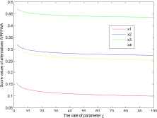
Figure 1 shows how the score values given by IVPFFPWA operator decrease according to the increasing χ. Moreover, from Figure 1, the following cases can be obtained:
- (1)
If χ ∈ (1, 12.88], then the order relation of alternatives Ai (i ∈ M4) is A4 ≻ A1 ≻ A3 ≻ A2, and the best alternative is A4. If χ ∈ (12.88, 50), then we obtain the ordering relation of Ai (i ∈ M4) as A4 ≻ A3 ≻ A1 ≻ A2.
- (2)
The score values
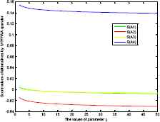
Score values obtained in the use of the IVPFFPWA operator.
The score value
- (i)
If χ ∈ (1, 12.88), then
- (ii)
If χ = 12.88, then
- (iii)
If χ ∈ (12.88, 50), then
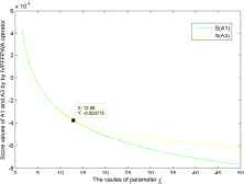
Score values of A1 and A3 obtained in the use of the IVPFFPWA operator.
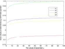
Figure 3 illustrates how the score values obtained with the IVPFFPWG operator increase in respect of the increasing χ, and more analysis are offered as following.
- (1)
When χ ∈ (0, 50), the ranking of Ai (i ∈ M4) is A4 ≻A3 ≻A1 ≻ A2, and the best alternative is invariably A4.
- (2)
The score values
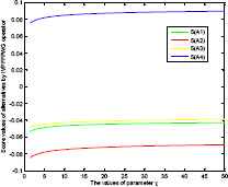
Score values obtained in the use of the IVPFFPWG operator.
Figures 4 and 5 show the deviations between the score values obtained by the IVPFFPWA operator and those obtained by the IVPFFPWG operator, from which we obtain
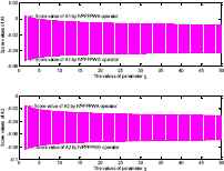
Score values of A1 and A2 obtained in the use of the IVPFFPWA/IVPFFPWG operator.
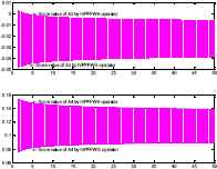
Score values of A3 and A4 obtained in the use of the IVPFFPWA/IVPFFPWG operator.
We use two generalized operators (IVPFFPWA/IVPFFPWG) and their limiting operators (IVPFPWA/IVPFPWQ/IVPFPWG) to obtain the score values of alternative A1. The details can be found in Figure 6. Consequently, the following ordering relation is obtained from Figure 6:
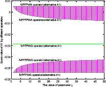
Score values of A1 by different operators.
Figure 6 illustrates the level of optimism and pessimism decreases when χ increases, and the decision maker’s attitude could be regarded as neutral when χ → ∞.
According to the previous analysis, it is observed that the associated parameter χ to the IVPFFPWG and the IVPFFPWA operators can be considered as a promising reflection of the attitude of DM. The DMs can obtain different score values of the collective overall preference values when different values of parameter χ are fixed in the sense that they can obtain different rankings of alternatives indicating their preferences. Therefore, the decision-making approaches with the IVPFFPWG and the IVPFFPWA operators are highly flexible and can provide DMs with more choices in handling different real-lief scenarios.
6.3. Comparative analysis
In the sequel, the proposed IVPFFP aggregation operators will be compared to several aggregation operators that were developed in 10,13,16 to evidence their superiority. Detailed analysis are provided in accordance with the performance of the compared aggregation operators given that they are used for the aggregation of individual decision matrices Dk (k ∈ T) in the context of MAGDM.
The three selected aggregation operators for comparison are briefly introduced in the first place. In Peng and Yang10, the weighted average (WA) and weighted geometric (WG) operators were accommodated to the Pythagorean fuzzy environment. The interval-valued Pythagorean fuzzy WA operator and WG operator, which are denoted separately by P-IVPFWA and the P-IVPFWG to distinguish themselves from the proposed ones, were developed to aggregate individual IVPF decision matrices. In Liang et al.13, based on the Algebraic operational laws10,11, the IVPFWA operator and IVPFWG operator were defined to aggregate individual decision matrices into a collective decision matrix. In Zhang16, the frank t-norm and s-norm were adopted as a basis for defining the interval-valued intuitionistic fuzzy frank weighted average (IVIFFWA) operator and the interval-valued intuitionistic fuzzy frank weighted geometric (IVIFFWG) operator, which were further used in the aggregation of individual IVIF decision matrixes.
The first comparison made is between the P-IVPFWA and P-IVPFWG operators and the IVPFFP operator. Recall that the generalized Pythagorean fuzzy aggregation operator was defined by Yager1,2 to gather a collection of PFNs satisfying the following characteristic:Agg = ηp ○ Aggd ○ ηp, where Agg and Aggd are dual with respect to the Pythagorean negation
- (i)
In the case that the P-IVPFWA operator was applied we have
- (ii)
In the other case that the P-IVPFWG operator was applied we obtain
The second comparison will be conducted for the IVIFFWA and IVIFFWG operators. According to Theorem 23, the IVPFWA and IVPFWG operators are essentially the respective special cases of the IVPFPWA and IVPFPWG operators. Likewise, the IVPFWA and IVPFWG operators are adopted to address the MAGDM problem in subsection 6.1 and the following decision results can be obtained.
- (i)
In the case that the IVPFWA operator was applied we have
- (ii)
In the other case that the IVPFWG operator was considered we have
The last comparison was made between Zhang16 and our proposal. Yager1,2 points out that all IFNs are PFNs, but not vice versa. Likewise, all IVIFNs are IVPFNs, but not the other way around. Therefore, the IVIFFWA and IVIFFWG operators in 16 can not be used to solve the aforementioned MAGDM problem. On the contrary, the IVPFFP operator proposed in this paper is capable of addressing the MAGDM problem provided as Example 5.1 in 16, and the following decision results can be obtained accordingly.
- (i)
If the IVPFFPWA operator instead of the IVIFFWA operator has been adopted, then we have
- (ii)
If the IVPFFPWG operator rather than the IVIFFWG operator has been adopted, then we get
The final score values changing with the varying parameter are shown in Figure 8. Despite the ranking of alternatives x2 and x4 obtained using our approach is different from that derived from the IVIFFWG operator, the best alternative selected is x3 in both cases. The reason that the ranking positions of (x2 and x4) get changed is because the IVPFFPWA and IVPFFPWG operators take into account the support function, and the scores of alternatives x2 and x4 are pretty close to each other. This is generally not the case for the IVIFFWA and IVIFFWG operators as the support function was not factored in.
Score values by IVPFFPWA operators.
Score values by IVPFFPWG operators.
In comparison to the several existing aggregation operators described above, the proposed IVPFFP aggregation operators present the following benefits in its implementation process.
- (1)
The convenience of expert weight elicitation. The IVPFFP operator can provide DM more flexibility in determining the weights of experts in the context of MAGDM. On the one hand, if the DM trusts the expert who provides evaluations completely and is allowed to determine the weight of the expert all on his/her own, then the support degree can be set as a constant, in which case the IVPFFPWA and IVPFFPWG operators degenerate to the IVPFFWA and IVPFFWG operator, respectively. This is a fact that can be reflected from Theorem 13(2) and Theorem 17(2). On the other hand, if the DM gets inadequate information at hand about the expert who provides evaluations, the expert weight elicitation depends entirely on the support function. In this case, the IVPFFPWA and IVPFFPWG operators reduce to the IVPFFPA and IVPFFPG operators, respectively, which can be observed in Theorem 13(1) and Theorem 17(1). Otherwise, the combination weight involving both subjective and objective approaches can be used to determine the aggregation weight of experts with the IVPFFWA and IVPFFWG operators.
- (2)
The variable parameter values indicating preference orientations.
Following the previous analysis conducted in subsection 6.2, it is observed that the adjustable parameter χ conforms to the DM’s preferences in the sense that the DM can determine the appropriate values of χ in accordance with their preference orientations.
- (3)
The expansion of domain for evaluation.
The IVPFFPWA and IVPFFPWG operators are able to deal with MAGDM problems with interval-valued Pythagorean fuzzy inputs, which is a benefit that the IVPFFWA and IVPFFWG operator do not share. It is as well convenient for DMs to adapt the IVPFFPWA and IVPFFPWG operators into MAGDM with interval-valued intuitionistic fuzzy inputs in the use of the idea raised in this paper.
7. Conclusions
In this study, we applied a special automorphism on the unit interval to construct an isomorphic Frank dual triple, which can be used to define the interval-valued Pythagorean Frank operations. We further revealed that these generalized operations include the existing operations for IVPFNs as special cases and discussed some fundamental properties of them. Subsequently, we proposed the IVPFFPWA and IVPFFPWG operators based on the proposed Frank operations and explored plenty of instrumental properties of the IVPFFPWA and IVPFFPWG operators. Several limiting cases of the proposed aggregation operators have as well been discussed in respect of the introduced adjustable parameter. We developed an IVPFFPWA (or IVPFFPWG) operator-based technique to deal with a classical MAGDM problem, provided an illustrative example to effectively verify the approach, and studied the influences of the adjustable parameter on the final aggregation results. The comparative analysis further demonstrated the superiority of the proposed aggregation techniques.
In future study, we are poised to pay more attention to the integration of IVPFNs with linguistic implication to foster their applications in the area of linguistic decision making33,34. Investigation on how varying associated weighting vectors will impact the final decision outputs under the interval-valued Pythagorean fuzzy environment will as well be a promising endeavor for future research35. Certain accuracy enhancements of the MAGDM with IVPFNs are expected to be achieved in the subsequent development of this study.
Acknowledgments
This work was supported by “the Fundamental Research Funds for the Central Universities” (Grant No. 2042018kf0006) and the Theme-based Research Projects of the Research Grants Council (RGC) (Grant No. T32-101/15-R), and partly supported by the Key Project of the National Natural Science Foundation of China (Grant No. 71231007), the National Natural Science Foundation of China (Grant No. 71373222), and the Open Fund of Key Laboratory of Hunan Province (2017TP1026).
References
Cite this article
TY  - JOUR
AU  - Yi Yang
AU  - Zhen-Song Chen
AU  - Yue-Hua Chen
AU  - Kwai-Sang Chin
PY  - 2018
DA  - 2018/06/07
TI  - Interval-valued Pythagorean Fuzzy Frank Power Aggregation Operators based on An Isomorphic Frank Dual Triple
JO  - International Journal of Computational Intelligence Systems
SP  - 1091
EP  - 1110
VL  - 11
IS  - 1
SN  - 1875-6883
UR  - https://doi.org/10.2991/ijcis.11.1.83
DO  - 10.2991/ijcis.11.1.83
ID  - Yang2018
ER  -