
A Three-Stage Based Ensemble Learning for Improved Software Fault Prediction: An Empirical Comparative Study
- DOI
- 10.2991/ijcis.11.1.92How to use a DOI?
- Keywords
- Software Fault Prediction; Software Testing; Ensemble Learning Algorithms; Feature Selection; Data Balancing; Noise Filtering
- Abstract
Software Fault Prediction (SFP) research has made enormous endeavor to accurately predict fault proneness of software modules, thus maximize precious software test resources, reduce maintenance cost and contributes to produce quality software products. In this regard, Machine Learning (ML) has been successfully applied to solve classification problems for SFP. However, SFP has many challenges that are created due to redundant and irrelevant features, class imbalance problem and the presence of noise in software defect datasets. Yet, neither of ML techniques alone handles those challenges and those may deteriorate the performance depending on the predictor’s sensitiveness to data corruptions. In the literature, it is widely claimed that building ensemble classifiers from preprocessed datasets and combining their predictions is an interesting method of overcoming the individual problems produced by each classifier. This statement is usually not supported by thorough empirical studies considering problems in combined implementation with resolving different types of challenges in defect datasets and, therefore, it must be carefully studied. Thus, the objective of this paper is to conduct large scale comprehensive experiments to study the effect of resolving those challenges in SFP in three stages in order to improve the practice and performance of SFP. In addition to that, the paper presents a thorough and statistically sound comparison of these techniques in each stage. Accordingly, a new three-stage based ensemble learning framework that efficiently handles those challenges in a combined form is proposed. The experimental results confirm that the proposed framework has exhibited the robustness of combined techniques in each stage. Particularly high performance results have achieved using combined ELA on selected features of balanced data after removing noise instances. Therefore, as shown in this study, ensemble techniques used for SFP must be carefully examined and combined with techniques to resolve those challenges and obtain robust performance so as to accurately identify the fault prone software modules.
- Copyright
- © 2018, the Authors. Published by Atlantis Press.
- Open Access
- This is an open access article under the CC BY-NC license (http://creativecommons.org/licences/by-nc/4.0/).
1. Introduction
The main reason for software failures are software faults, located in software modules. This critically affect the reliability of software product and user satisfaction, which ultimately degrade company efficiency. However, the growing demands for quality software in different industry have been increasing. Nevertheless, software may have thousands of modules. Its resource consuming to allocate human and financial resources to go through all modules exhaustively to identify faulty prone modules. Thus, the scarcity of testing resources and the demand for high quality software products have been igniting the Software Fault Prediction (SFP) research area. Thereby the quality can be cautiously inspected and undertaken before releasing the software. SFP is targeted to inspect and detect fault proneness of software modules and help to focus more on those specific modules predicted as fault prone so as to manage resources efficiently and reduce the number of faults occurring during operations. In this regard, statistical and Machine Learning (ML) techniques have been employed for SFP in most studies [3–14]. On the other hand, from ML techniques, Ensemble Learning Algorithms (ELA) have been demonstrated to be useful in different areas of research [7, 15–18], where all of them have confirmed that ELA can effectively solve classification problems with better performance when compared with an individual classifier. As illustrated in the literatures [6, 14, 32, 35], it’s more like, to make wise decisions, people may counsel many experts in the area and take consideration of their opinions rather than only depend on their own decisions. Likewise, in fault prediction, a predictive model generated by ML can be considered as an expert. Therefore, a good approach to make decisions more accurately is to combine the output of different predictive models. So that, all can improve or at least equal to the predictive performance over an individual model [6, 14, 32, 35]. Therefore, in this study, we develop a new framework to compare eminent ELA, namely, Bagging (BaG), AdaBoost.M1 (AdB), Random Forest (RaF), LogitBoost (LtB), MultiBoostAB (MtB), RealAdaBoost (RaB), Stacking (StK), StackingC (StC), Vote (VoT), Dagging (DaG), Decorate (DeC), Grading (GrD), and Rotation Forest (RoF) with J48 Decision Tree (DTa) as a base classifier for all ELA except that Decision Stump (DSt) is used as a base classifier for LtB. In addition to that, we use McCabe and Halstead Static Code Metrics [19, 22] datasets for experimental analysis.
In addition to that, in the literature, it is widely claimed that building ensemble classifiers from preprocessed datasets and combining their predictions is an interesting method of overcoming the individual problems produced by each classifier [8, 16, 18, 25], but neither of these learning techniques alone solve the major challenges (problems) in SFP, such as class imbalance problems [16, 26], the existence of redundant and irrelevant features [10, 26] and the presence of noise [39, 41] in defect datasets. Moreover, as observed in the literature [2, 5, 12, 13, 26, 43, 44], the classification performance of a learner is directly influenced by the quality of the training data used. Real world datasets usually contain corrupted data that may hinder the interpretations, decisions, and therefore, the ensemble classifiers built from that data is less accurate. Thus, to deal with these issues, an ensemble based combined framework has to be designed specifically. Therefore, in this study, our plan is to combine ELA with Feature Selection (FS) [9, 12–14, 20, 21, 45–47], Data Balancing (DB) [11, 20, 23–25, 47] and Noise Filtering (NF) [36–42, 44] techniques. FS is carried out by removing less important and redundant features, so that only beneficial features are left for training the models. The complexity of the ELA could be reduced and the learned knowledge may be more compact and easily understood. ELA could be faster and more cost-effective and the performance of ELA could be improved. Therefore, in Stage 1, this study employs Information Gain (IG) FS technique, which has been proven good in different SFP studies [10, 14, 26].
On the other hand, the nature of software defect datasets consists of Fault-Prone (FP) and Not-Fault-Prone (NFP) modules and class imbalance problems occur where one of the two classes having more sample than other classes. It has been seen that these datasets (see Table I) are highly skewed toward the NFP modules and the number of FP modules are relatively very small. Even though, FP (minority) samples are those that rarely occur but very important, however learners are more focusing on classification of NFP samples while ignoring or misclassifying minority samples. Thus, DB is carried out to resolve the skewed nature of defect datasets, so that building SFP models on balanced data could improve ELA performance. In view of that, the ML community has addressed the imbalance nature of defect datasets in two ways. One is to assign distinct costs to training examples. The other is to re-sample the original dataset, either by oversampling the minority class and/or under-sampling the majority class [11, 23]. As shown in different studies [23, 25, 26, 42], balancing data using Synthetic Minority Oversampling Techniques (SMOTE) gives better classification performance. Therefore, in Stage 2, this study explores the algorithm of SMOTE for building SFP models with datasets that suffer from class imbalance.
| Dataset | #Attr | #Ins | #NFP | #FP | %NFP | %FP |
|---|---|---|---|---|---|---|
| ar1 | 29 | 121 | 112 | 9 | 92.56% | 7.44% |
| ar3 | 29 | 63 | 55 | 8 | 87.30% | 12.70% |
| ar4 | 29 | 107 | 87 | 20 | 81.31% | 18.69% |
| ar5 | 29 | 36 | 28 | 8 | 77.78% | 22.22% |
| ar6 | 29 | 101 | 86 | 15 | 85.15% | 14.85% |
| CM1′ | 37 | 344 | 302 | 42 | 87.79% | 12.21% |
| JM1′ | 21 | 9593 | 7834 | 1759 | 81.66% | 18.34% |
| KC2 | 21 | 522 | 415 | 107 | 79.50% | 20.50% |
| kc3 | 39 | 194 | 158 | 36 | 81.44% | 18.56% |
| MC1″ | 38 | 1988 | 1942 | 46 | 97.69% | 2.31% |
| MC2′ | 39 | 127 | 83 | 44 | 65.35% | 34.65% |
| MW1′ | 37 | 264 | 237 | 27 | 89.77% | 10.23% |
| pc1 | 37 | 705 | 644 | 61 | 91.35% | 8.65% |
| pc2 | 36 | 745 | 729 | 16 | 97.85% | 2.15% |
| PC3′ | 37 | 1125 | 985 | 140 | 87.56% | 12.44% |
| pc4 | 37 | 1458 | 1280 | 178 | 87.79% | 12.21% |
| pc5 | 38 | 17186 | 16670 | 516 | 97.00% | 3.00% |
A description of datasets.
Moreover, the presence of noise in defect datasets is a common challenge that produces several negative consequences in fault prediction problems. The most frequently reported consequence is that it negatively affects prediction accuracy and complexity of the classifier built in terms of time, size and interpretability [36, 38, 40, 43, 44]. Class noise occurs when an example is incorrectly labeled [36]. In addition to subjectivity during labeling process, the class noise can be attributed to data entry errors, or inadequacy of the information used to label each example. In the literature, two approaches have been proposed to deal with noise [37, 38]: algorithm level and data level approaches. Accordingly, two types of noise are distinguished [38]: attribute noise and class noise. Attribute noise affects the values of one or more attributes of examples in a dataset. Class noise is produced when the examples are labeled with the wrong classes and it compromises classification performance more than attribute noise [37–39]. For this reason, this paper focuses on class noise, aiming at removing those wrongly labeled examples from the defect datasets, so that building SFP models on noise filtered data could improve ELA performance. Therefore, in Stage 3, this study employs Iterative Noise Filter based on the Fusion of Classifiers (INFFC) [37] for building SFP models to resolve the presence of noisy instances from defect datasets. In this paper, class noise refers to misclassifications.
As discussed in the literature, it’s generally confirmed that building classifiers from preprocessed datasets produce better results than building on original data for many reasons. Hence, this statement is usually not supported by thorough empirical studies considering problems in combined implementation with resolving different types of challenges created in SFP due to large number of features, nature of class imbalance and presence of noisy in defect datasets. Therefore, the objective of this paper is to conduct large scale comprehensive experiments to study the effect of resolving those challenges in SFP in three stages, which consider important features selection, well balanced class distribution and noisy instance filtering in order to improve the practice and performance of SFP. Thus, this paper is motivated to independently examine and compare eminent ELA and its interactions with preprocessing stages. Accordingly, a new three-stage based combined ensemble framework that efficiently handles those challenges in a combined form is proposed. Hence, the primary contribution of this study is the empirical comparative analysis of multiple ELA in combination with FS, DB and NF in different stages and realizing its contributions to more accurately identify FP modules for software product quality inspection. Interestingly, the proposed framework has combined ELA on selected features of balanced data after removing noise instances, which constitutes a major contribution credited to this study. Moreover, statistical techniques confirmed that from Stage 1 through Stage 3, our combined techniques significantly contribute to performance improvements in each stage, which is the secondary contribution attributed to this study.
2. Related Work
In this section, we focus on the studies that have attempted to address classification problems using ensemble and preprocessing techniques to build fault-proneness prediction models.
Studies typically produce fault prediction models which allow Software Engineers to focus development activities on FP code, thereby improving software quality and making better use of resources [9, 25, 26, 28, 29]. In this regard, Laradji [8] demonstrated the effectiveness of using average probability ensemble (APE) that consists of seven carefully devised learners. They also showed the positive effects of combining feature selection and ensemble learning on the performance of faulty prediction. The experimental result shows that selecting few quality features makes much higher AUC than otherwise. Khoshgoftaar et al. [18] investigated FS, under-sampling with AdaBoost algorithm exhibited the robustness of combined techniques. Particularly high performance results have exhibited with and their main drive was to make a comparison between repetitive sample FS and individual FS. And they confirmed that using boosting is effective in improving classification performance. On the other hand, Shanthini et al. [15] developed a bagging ensemble with Support Vector Machine (SVM) as a base learner for SFP. They showed that the proposed ensemble of SVM is superior to individual approach for SFP. It is also important to note that both of these studies don’t consider employing multiple ensemble approaches and filter noise so as to identify the techniques that are more efficient to predict faulty modules.
As discussed earlier, the ELA is known to increase the performance of individual classifiers, but neither of these ensemble techniques alone solves the existence of irrelevant features, class imbalance and noise in defect datasets. To deal with these issues we have realized that the performance of ELA can be increased by keeping the quality of software defect datasets, which can be done by applying either FS, resolving class imbalance problem and/or filtering noise instances [12, 13, 18, 25, 26, 41, 42, 44, 47] from defect datasets. In this regard, Liu et al. [45] made a comprehensive survey of FS algorithms. Shivaji et al. [12] investigated multiple FS using NB and SVM classifiers. Hall et al. [46] presented a comparison of six attribute selection techniques that produce ranked lists of attributes. The experimental results show that in general, attribute selection is beneficial for improving the performance of learning algorithms. However, there is no single best approach for all situations. Liu et al. [47] proposed a two-stage data preprocessing approach to improve the quality of software datasets used by classification models for SFP. In the FS stage, they proposed an algorithm which involves both relevance analysis and redundancy control. Their approach enhances the prediction performance of the classifiers. Wang et al. [13] presented a comprehensive empirical study to evaluate 17 ensemble of feature ranking methods including 6 commonly-used feature ranking techniques and 11 threshold-based feature ranking techniques. Experimental results indicated that ensemble of very few rankers are effective and even better than ensemble of many or all rankers. As noticed, these studies didn’t employ different ensemble techniques; perform DB (except [47]) and NF to resolve class imbalance issues and filter noise from the defect datasets.
In ML field, most standard algorithms assume or expect balanced class distributions or equal misclassification costs. Thereby, there is no significant difference between the number of samples in the majority and minority classes. However, when presented with complex imbalanced data sets, these algorithms fail to properly represent the distribution of the data and resultantly provide unfavorable accuracies across the classes of the data [2, 5, 11, 23–26, 47]. Thus, in recent years, the imbalanced learning problem has drawn a significant amount of interest in Software Engineering research area, particularly in SFP. For example, Wang et al. [2] investigated different types of class imbalance learning methods, including resampling techniques, threshold moving, and ensemble algorithms. Then improved the performance of the AdaBoost.NC algorithm, and facilitated its use in SFP, in the way that AdaBoost.NC adjusts its parameter automatically during training without the need to predefine any parameters. The experimental result shows that it’s more effective and efficient than the original AdaBoost.NC. Khoshgoftaar et al. [5] presented an empirical study of learning when very few examples of one class are available for training models. Specifically, they addressed the issue of how many majority class examples should be included in a training dataset when the minority class is rare. They presented a very practical scenario where few positive class examples are available, while negative class examples are available in abundance. The findings indicated that the optimal class distribution when learning from data containing rare events is approximately 2:1 (majority: minority). In the same work, Liu et al. [47] used data sampling techniques to resolve the class distribution ration in their two-stage data preprocessing approach. The experimental result shows the contribution of DB for classification performance improvement. Song et al. [48] conducted a comprehensive experiment to explore the effect of using imbalanced learning to predict FP software components by exploring the complex interaction between type of imbalance learning, classifiers, and input metrics. The experimental result shows imbalance in software defect data clearly harms the performance of standard learning even if the imbalance ratio is not severe. Imbalance learning methods are recommended when the imbalance ratio is greater than 4. The particular choice of classifiers and imbalance learning methods is important. Moreover, in [23], García et al. presented a thorough empirical analysis of the effect of the imbalance ratio and the classifier on the effectiveness of resampling strategies when dealing with imbalanced data. The experiments have used 17 datasets 8 classifiers and 4 resampling methods. Besides, the performance has been evaluated by means of four different metrics. Experimental results have shown that, in general, over-sampling performs better than under-sampling for data sets with a severe class imbalance. In addition, Chubato et al. [26] investigated the contribution of combined implementation of sampling as one part of preprocessing techniques for SFP, and particularly they employed SMOTE to resolve the class distribution problem. The experimental result shows the contribution of DB to improve the learning algorithms. Chawla et al. [11] proposed an over-sampling approach in which the minority class is over-sampled by creating “synthetic” examples rather than by over-sampling with replacement. The minority class is over-sampled by taking each minority class sample and introducing synthetic examples along the line segments joining any/all of the k minority class nearest neighbors. Depending upon the amount of over-sampling required, neighbors from the k nearest neighbors are randomly chosen. Inspired by Chawla’s powerful method that has shown a great success in various applications [11, 24], most of the imbalanced learning studies and some of the above works has successfully used to attain their study goal. As noticed, except [26, 47], many of the study didn’t systematical combined this powerful method with other preprocessing techniques that has equivalent contribution to solve the major challenges of SFP so as to improve the prediction performance. Therefore, this paper systematically combines this method with other different preprocessing techniques to combat the major challenges mentioned in this study.
Moreover, the impact of the presence of class noise in the dataset on the classification problem has been analyzing in different literatures [36, 37, 39, 40–42, 44,]. For example, Sáez et al. [37] proposed a noise filtering method that combines several filtering strategies in order to increase the accuracy of the classification algorithms used after the filtering process. They compared their method against other well-known filters over a large collection of real-world datasets with different levels of class noise. INFFC outperformed the rest of noise filters compared. Khoshgoftaar et al. [41] investigated the quality of the training defect dataset improvement by removing instances detected as noisy by the Partitioning Filter. They first split the fit dataset into subsets, and then induced different base learners on each of these splits. The predictions are combined in such a way that an instance is identified as noisy if it is misclassified by a certain number of base learners. Two versions of the Partitioning Filter are used: Multiple-Partitioning Filter and Iterative-Partitioning Filter. The results show that predictive performances of models built on the filtered fit datasets and evaluated on a noisy test dataset are generally better than those built on the noisy (un-filtered) fit dataset. Catal et al. [44] proposed a noise detection approach that is based on the threshold values of software metrics, and validated their technique using NASA datasets. Experimental result shows their approach is very effective for detecting noisy instances, and the performance of the SFP model is improved. As noticed, these studies didn’t employ different ensemble techniques and perform FS and DB to select more suitable features and resolve class imbalance issues. As the defect datasets are suffering from class imbalance problem and the presence of irrelevant and redundant features, these preprocessing stages (FS and DB) are crucial to enhance the predictive power of ELA so as to accurately identify FP modules. Therefore, to the best of our knowledge, no research attempt has been made on combined implementation of multiple ELA with FS, DB and NF (in our case, IG, SMOTE and INFFC) concepts together for SFP.
Having this gap in mind, which has not been addressed by many studies, we design a new framework that follows three stages step by step. Firstly, in Stage 1, we employ FS with multiple ELA to build models and identify techniques that better predict fault proneness of a module using selected feature sets. Secondly, in Stage 2, we apply DB technique on the best features selected and build a model using ELA to identify techniques that predict fault proneness of software modules more efficiently after employing combined FS and DB, and also to realize the contribution of proper class distribution for performance improvements of ELA. Finally, we combine three techniques together (FS, DB and NF). Filtering noise from balanced data of selected features has done in Stage 3. Then empirical analysis and comparisons are made among ELA and between stages (Stage 1, Stage 2, and Stage 3) to realize whether removing noise could contribute the performance of ELA or not, which in turn empower the predictive performance of ELA for more accurately predicting FP modules. Moreover, we employ statistical techniques to compare the first, second and the third stage as well as ELA within each stage results using AUC to see their significant contribution to accurately identify the FP modules. Furthermore, to conclude our study we use the average result of different performance metrics such as Accuracy, F-Measure, Root Mean Squared Error (RMSE) and Elapsed Time Training (ETT). Details of our new three stage based combined ensemble learning framework for improved SFP are presented in Section III.
3. A Three-Stage Based Ensemble Framework For Improving SFP
3.1. Proposed Framework
An ensemble based combined framework for improved SFP is shown in Figure 1. We follow three stages to attain the objective of the study. Therefore, in this section, we introduce our proposal to alleviate the challenges mentioned in this study so as to remove redundant and irrelevant features, resolve class imbalance problem and filter noise from the defect datasets. As mentioned above, our proposed framework hybridizes ELA with three stage preprocessing techniques. One-way ANOVA is used to examine the significance level of the differences in SFP model performances. Tukey’s Honestly Significant Difference (HSD) tests is used for multiple pairwise comparisons, to find out which pairs of means (in each stages) are significantly different, and which are not. Supplementing the statistical analysis, we also reflect the average ranking of the algorithms in order to show at a first glance how good an ELA performs with respect to the rest in the comparison. The rankings are computed by using the AUC result of each algorithm in every dataset in each stage. The first rank of each dataset is assigned to the best performing ELA with highest AUC as a winner. Then the top 3 ELA for each datasets are selected accordingly based on their AUC results. Finally, the average ranking of algorithms is computed by the mean value of different Performance Evaluation (PE) index results among all 17 datasets.

A Three-Stage Based Ensemble Framework for Improving SFP
In Stage 1, we perform FS using IG evaluation methods based on Ranker search methods for all datasets used in this study to identify useful features for ensemble learning. The input of the framework for this stage is top ranked features from all datasets. Then we build the SFP models on the selected features using 13 prominent ELA (BaG, AdB, RaF, LtB, MtB, RaB, StK, StC, VoT, DaG, DeC, GrD, and RoF) and two base classifiers, DTa for all ELA except DSt for LtB which is carried out by running a 10-fold cross-validation. Each cross-validation run is repeated 10 times to avoid bias due to a lucky or unlucky data split. Then the results are captured using AUC, Accuracy, F-Measure, RMSE and ETT PE criteria. As shown in Figure 1, this strategy serves as to compare ELA performance. Also we use these results for further comparable reference in the subsequent performance experiments. In this study, we do not present the classification results based on the complete set of software defect datasets, because in a recent study [26], it was demonstrated that SFP models built on fewer software metrics (after FS) performed generally better than models based on the complete set of software metrics.
In Stage 2, we resolve the data skewness problem using SMOTE algorithm on the selected features of the defect datasets. To get reasonably balanced data for ensemble classification, we make the target ration for NFP and FP module as recommended to be 65% and 35%, respectively [5]. As shown in Figure 1, this stage serves as to demonstrate performance improvement by combining both IG and SMOTE with ELA, and to realize efficient ensemble fault predictor, which will be used to compare with the previous performance experiment. Also we use these results as comparable reference in the subsequent performance experiment.
In Stage 3, we resolve the class noise problem using INFFC methods from defect datasets which is applied on the dataset that is with balanced class distribution and important features selected. As shown in Figure 1, this stage serves as to combine all three techniques (IG, SMOTE and INFFC) together to clean defect datasets and empower ELA so as to more accurately predict the fault proneness of modules as well as to prove the performance improvement, realize the efficient ensemble classifier and use these results to compare with the previous performance experiment.
Finally, we make comparison between the combined ELA in Stage 1, Stage 2 and Stage 3 based on different PE criteria and statistical techniques to realize performance improvements and see the significant contribution of resolving the challenges of SFP in combined form.
The experimental procedures are presented in Algorithm 1. It summarizes overall combined approaches. Step 1 to 9 defines the datasets used, the preprocessing techniques employed, ELA implemented, base learners used as well as the number of folds and repeating experiment. In all three stage experiments, we used 10 folds and repeated the experiments 10 times. Step 10 to 25, calculates the probability of attributes, entropy, expected information required, information gained by attributes, then rank and sort attributes based on the information gain, and finally select top ranked attributes. Step 26 to 37, use datasets with only top selected features as input, define FP and NFP instances, determine rates to synthetically create FP instances based on the required percentage of FP instances, and then choose one of FP instances randomly from k - nearest neighbors, and introducing synthetic examples along the line segments joining any/all of the minority class nearest neighbors. Step 38 to 42, define classifiers used for fusion, and then three steps of noise filtering are carried on: as a Preliminary Filtering balanced datasets are used for fusion classifier based noise filter, as Noise Free Filtering balanced datasets together with partially clean sets are used for fusion classifier based noise filter, as Final Removal of Noise calculate the noise score from noise sets and remove the noise instances and generate noise free datasets. Step 43 to 55, input cleaned datasets, generate 10 folds of each datasets, repeat the experiments 10 times, predict fault proneness of the modules in each stage, and evaluate the performance of ELA on test datasets.
| 1 | Datasets ← {D1, D2, ..., Dn}; /*defect datasets*/ |
| 2 | FS ← IG; /*redundant and irrelevant feature removing method*/ |
| 3 | DB ← SMOTE; /*Data Balancing method*/ |
| 4 | NF ← INFFC; /*Noise Filtering method*/ |
| 5 | ELA ← {BaG, AdB, RaF, LtB, MtB, RaB, StK, StC, VoT, DaG |
| 6 | DeC, GrD, RoF};/*Ensemble Learning Algorithms*/ |
| 7 | BaseLearner ← {DTa, DSt}; |
| 8 | R ← 10; /*the number of repeating experiment*/ |
| 9 | N ← 10; /*the number of folds*/ |
| 10 | for each D ∊ Datasets do |
| 11 | Pi ← |Ci,D|/|D|/ *probability of arbitrary tuple blongs to class Ci*/ |
| 12 |
|
| 13 | |
| 14 | InfoGain(A) ← Info(D) – Info (D) / *information gained by A */ |
| 15 | for each A ∊ D do / * attiribute or feature selection */ |
| 16 | rankOfA ← InfoGain (A) / * the highest ranked attribute A is the one with the largest information gain */ |
| 17 | rankOfA '[ ] ← {rankOfA1, rankOfA2, … rankO fAn}; |
endfor |
|
| 18 | for I = 0 to length-1 do /* sort A based on InfoGain(A)*/ |
| 19 | highRank = I; |
| 20 | for J = I + 1 to length-1 do |
| 21 | if rankOfA '[J] > rankOfA '[highRank] |
| 22 | highRank = J; |
endif |
|
endfor |
|
| 23 | Temp = rankOfA '[I]; rankOfA '[I] = rankOfA '[highRank]; |
| 24 | rankOfA '[highRank] = Temp; |
endfor |
|
| 25 | selectedDFeatures ← top[log2n] + class A; /* selecting top ranked*/ |
| 26 | D' ← selectedDFeatures; |
| 27 | Smino ∊ D'; /* Smino is a subset of # FP ins tan ces */ |
| 28 | Smajo ∊ D'; /* Smajo is a subset of # NFP ins tan ces */ |
| 29 | Pmajo ← recommended/required percentage of Smajo; |
| 30 | xi ∊ Smino; /* is the # FP ins tan ce underconsideration its one of the k - nearest neighbors for xi: xi∧ ∊ Smino*/ |
| 31 | k ← 5; /*set 5 as k-nearest neighbors for each example xi ∊ Smino */ |
| 32 | δ ∊ [0,1]; /* is a uniformal distribution random variable */ |
| 33 |
|
| 34 | for ∀ xi ∊ Smino |
| 35 |
|
| 36 |
|
endfor |
|
| 37 | balancedData ← D' + xnewMino;/* balanced data on selected features */ |
| 38 | FC ← {C4.5, 3-NN, LOG}; /*Classifiers used in FC-based filter */ |
| 39 | for ∀ ci ∊ FC |
| 40 | partiallyCleanSet ← FCbasedFilter(balancedData); /*Preliminary filtering*/ |
| 41 | noisySet ← FCbasedFilter(balancedData, partiallyCleanSet); /*Noise Free Filtering*/ |
| 42 | noiseFreeDSet ← noiseScore(noisySet); /*Final removal of noise*/ |
endfor |
|
| 43 | preprocessedData ← {selectedDFeatures, balancedData, noiseFreeDSet}; |
| 44 | for ∀ pdi ∊ preprocessedData |
| 45 | for each times ∊ [1, R] do /*R times N-fold cross-validation*/ |
| 46 | foldData ← generate N folds from pd; |
| 47 | for each fold ← [1, N] do |
| 48 | testData ← foldData[fold]; |
| 49 | trainingData ← pd - testData; |
| 50 | for each combELA ← ELA do /*evaluate combined ELA */ |
| 51 | faultPredictorStage1 ← combFSELA(trainingData); |
| 52 | faultPredictorStage2 ← combDBFSELA(trainingData); |
| 53 | faultPredictorStage3 ← combNFDBFSELA(trainingData); |
| 54 | V ← evaluate combined ELA on testData; |
| 55 | predictorPerformance ← choose the class that receives the highest V as the final classification; |
endfor |
|
endfor |
|
endfor |
|
endfor |
Experimental Procedure
3.2. Feature Selection
The goal of FS is to choose a subset Xs of the complete set of input features X={x1, x2, …, xM} and these features are very valuable for analysis and future prediction. So that the subset Xs can predict the output Y with accuracy comparable to or better performance than that of using the complete input set X with a great reduction of the computational cost [12, 13, 21]. Thus in this study we employ Information Gain (IG) FS, which has been proven good in SFP studies [10, 26].
Information Gain (IG): the IG measure is based on pioneering work by Claude Shannon on information theory, which studied the value or “information content” of messages. IG FS selects the attribute with the highest information gain. Let Pi be the probability that an arbitrary tuple in D belongs to class Ci, estimated by |Ci,D|/|D|. Therefore, expected information (entropy) required to encode an arbitrary class distribution in D is given by Info(D) (Step 12, Algorithm 1). Info(D) is just the average amount of information required to identify the class label of a tuple in D. Note that, at this point, the information we have is based solely on the proportions of tuples of each class. Info(D) is also known as the entropy of D.\
If A is a set of attributes, the number of bits required to encode a class after observing an attribute is given by InfoA(D) (Step 13, Algorithm 1). The term |Dj|/|D| acts as the weight of the jth partition. InfoA(D) is the expected information required to classify a tuple from D based on the partitioning by A. The smaller the expected information required, the greater the purity of the partitions.
The highest ranked attribute A is the one with the largest IG. Information gained by an attribute A is given by InfoGain(A) (Step 14, Algorithm 1). Therefore, IG is defined as the difference between the original information requirement (i.e., based on just the proportion of classes, (Step 12, Algorithm 1)) and the new requirement (i.e., obtained after partitioning on A, (Step 13, Algorithm 1)). That is in Step 14, Algorithm 1. In other words, InfoGain(A) tells us how much would be gained by branching on A. Thus, it’s the expected reduction in the information requirement caused by knowing the value of A [6, 14]. After computing IG, in Stage 1, we employ a ranker method that ranks attributes based on the gained value by sorting from the most informative to least informative. Then the top [log2n] (n is the number of independent features) attributes with highest IG are selected and the class attribute is included to get improved data to build combined ensemble based SFP models.
3.3. Class Imbalance and Its Solution
A dataset is imbalanced if the classification categories are not approximately equally represented. Often software defect datasets are composed of NFP instances with only a small percentage of FP instances. ML community has addressed the issue of class imbalance in two ways. One is to assign distinct costs to training instances [11]. The other is to re-sample the original dataset, either by over-sampling the minority class and/or under-sampling the majority class. In this study, we employ the special form of over-sampling technique, called SMOTE [11, 23]. It’s a powerful technique that has demonstrated remarkable contribution in various applications [23–26]. Thus, Stage 2 deals with data skewness using this technique. The main idea in SMOTE is to insert man-made hypothesized samples between a minority sample and its near neighbors in such a way that for every sample in the minority xi, search its k nearest neighbors and choose one of them randomly as xi^. Then a liner interpolation is fulfilled randomly to produce a new sample called XnewMino (Step 36, Algorithm 1). Finally, this step is continua n times for each instance of the entire minority instance xi, where n=p/100 and p is used as the amount of over-sampling rate required to balance the dataset. To get a reasonably balanced class distribution for classification, we make the target ration for NFP and FP module as recommended to be 65% and 35%, respectively [5]. Step 33 of Algorithm 1 computes and determines the over-sampling rate (in percentage) of minority class given the recommended target rate or required amount of class distribution.
3.4. Noise Filtering
Even though several noise filtering schemes are proposed in the literature [37, 41, 44], this study employs the INFFC. The filtering is based on the fusion of the predictions of several classifiers used to detect the presence of noise following iterative noise filtering scheme and introduce a noisy score to control the filtering sensitivity to remove more or less noisy examples according to the necessities. Thus, it combines three noise filtering paradigms: the usage of ensemble for filtering, the iterative filtering and the computation of noise measures. Therefore, in Stage 3, this study removes noisy examples in multiple iterations based on the fusion of classifiers.
3.5. Performance Evaluation
In this study, we employ accuracy which has been the most commonly used empirical measure. This combines both positive and negative class independent measures of classification performance. The accuracy formula is shown in Equation 1.
However, in the framework of imbalanced datasets, only accuracy is no longer a proper measure. For this reason, when working in imbalanced domains, there are more appropriate metrics to be considered in addition to accuracy. Another way to combine these measures and produce an evaluation criterion is to use the Area Under the Receiver Operating Characteristic (ROC) Curve (AUC) [34]. The ROC curves graph TPrate on the y-axis versus the FPrate on the x-axis. It is a tool for visualizing, organizing and selecting classifiers based on their tradeoffs between benefits (TPrate) and costs (FPrate) [33]. Thus, it’s not possible for classifiers to increase the number of TPrate without increasing the FPrate. As a result, it has got growing attention in different studies [2, 10–13]. Therefore, in addition to accuracy, we employ this popular technique for the evaluation of combined ELA in SFP problems. The AUC formula is shown in Equation 2.
Moreover, to conclude our study we use the average result of different performance metrics such as accuracy, F-Measure, RMSE and ETT. The precision and recall are often employed together in tasks that regard one class as being more important than the other. However, one single metric is still insufficient because a better recall sometimes means that the precision is not good enough. Therefore, we need a metric that can reflect the performance of algorithms better. Thus, a metric that harmonizes the average of precision and recall is called F-measure. It reaches its best value at 1 (perfect precision and recall) and worst at 0. The F1 score formula is shown in Equation 3.
RMSE is a commonly used measure of the differences between values predicted by a model and the values actually observed. The RMSE formula is shown in Equation 4.
The performances of the combined ELA are also compared with ETT. It’s a time measure for the entire training process based on processing all instances in the training data. We consider only the training time as we have employed 10-fold cross-validation, and the training instances are much bigger than the test instances.
4. Experimental Design
During the experiments, the performance evaluation is carried out by running a 10-fold cross-validation. Each cross-validation run is repeated 10 times to avoid bias due to a lucky and unlucky data split, approximately equal size split. For 10 times, 9 folds are picked to train the models and the remaining fold is used to test them, each time leaving out different fold. Based on IG, attributes are ranked then following the recommendation from literatures, we select the top [log2n] (n is the number of independent features) attributes and class attribute is included to yield final datasets. In the literature, a software engineering expert with more than 20 years’ experience recommended selecting [log2n] number of metrics for software quality prediction. In addition to that, a preliminary study showed that [log2n] is appropriate for various learners [13].
As discussed under Section III (A), the proposed ensemble based combined framework is implemented step by step following three stages. The performances of 13 ELA are evaluated against each other on each dataset over using 17 publicly available software defect datasets. Employed algorithms and statistical techniques are performed using WEKA version 3.8 [27] and Mathlab 2014a. The final comparison is based on using the average result of AUC, Accuracy, F-Measure, RMSE and ETT measures.
Datasets: the selected 17 datasets are the latest and cleaned versions, from publicly accessible PROMISE repository of NASA software projects [1]. These datasets have been widely used by many studies [29]. Table I summarizes some main characteristics of the selected datasets, where #Attr refers to the number of attributes, #Ins refers to the number of instances, #NFP refers to the number of negative instances, #FP refers to the number of positive instances, %NFP refers to the percentage of negative instances and %FP refers to the percentage of positive instances. Note that data imbalance is consistently observed in all datasets. These, datasets consist of McCabe and Halstead Static Code Metrics. McCabe and Halstead metrics attempt to objectively characterize code features that are associated with software quality. Their measures are “module” based where a “module” is the smallest unit of functionality. McCabe [22] argued that codes with complicated pathways are more error-prone. His metrics therefore reflect the pathways within a code module. His metrics are a collection of four software metrics such as Cyclomatic Complexity, Essential Complexity, Design Complexity and LOC. Whereas, Halstead argued that code which is hard to read is more likely to be fault-prone [10]. Halstead metric estimates the complexity by counting the number of concepts in a module, for instance, the number of unique operators/operands. His metric falls into three groups, such as Base Measures, Derived Measures, and LOC Measures. The value of using static code metrics to build SFP models has been empirically illustrated by Menzies et al. [10], who stated that static code metrics are useful, easy to use, and widely used.
5. Analysis and Discussions
In this section, we present the experimental analysis and comparative discussions based on the objective of the study. Performance comparison among 13 prominent ELA combined with FS technique (in our case IG), data imbalance problem solution (in our case SMOTE) and NF technique (in our case INFFC) presented in the following figures and tables. The results are based on the performance of ELA combined with IG FS; ELA combined with both IG and SMOTE; and finally ELA combined with both IG, SMOTE and INFFC. Table II to Table VII summarize the ELA performances in terms of AUC across three stages (Stage 1 through Stage 3). Each value presented is the average over the 10 runs of 10-fold cross-validation. The last row shows the winner, top 3 and average performance of the ELA in each stage over the 13 ELA, two base learners and across 17 datasets. Moreover, the average and statistical results using Accuracy, F-Measure, RMSE and ETT measures are presented in Table VIII to Table XII.
| Source | SS | df | MS | F | Sig. |
|---|---|---|---|---|---|
| Columns | 1.1075 | 14 | 0.07911 | 6.1257 | 0.000 |
| Error | 3.0993 | 240 | 0.01291 | ||
| Total | 4.2067 | 254 |
One-way ANOVA Results of Stage one.
| Source | SS | df | MS | F | Sig. |
|---|---|---|---|---|---|
| Columns | 0.40974 | 14 | 0.02927 | 3.3087 | 0.000 |
| Error | 2.1229 | 240 | 0.00885 | ||
| Total | 2.5326 | 254 |
One-way ANOVA Results for Stage Two.
| Source | SS | df | MS | F | Sig. |
|---|---|---|---|---|---|
| Columns | 0.1804 | 14 | 0.01289 | 11.9501 | 0.000 |
| Error | 0.25878 | 240 | 0.00108 | ||
| Total | 0.43918 | 254 |
One-way ANOVA Results for Stage Three.
| Dataset | BaG | RaF | AdB | LtB | MtB | RaB | StK | StC | VoT | DaG | DeC | GrD | RoF | DTa | DSt |
|---|---|---|---|---|---|---|---|---|---|---|---|---|---|---|---|
| ar1′ | 0.755 | 0.803 | 0.744 | 0.680 | 0.734 | 0.752 | 0.499 | 0.511 | 0.491 | 0.500 | 0.784 | 0.497 | 0.566 | 0.491 | 0.571 |
| ar3′ | 0.834 | 0.834 | 0.824 | 0.799 | 0.836 | 0.828 | 0.540 | 0.850 | 0.850 | 0.500 | 0.815 | 0.834 | 0.848 | 0.850 | 0.793 |
| ar4′ | 0.833 | 0.828 | 0.794 | 0.858 | 0.814 | 0.792 | 0.640 | 0.716 | 0.716 | 0.827 | 0.857 | 0.661 | 0.763 | 0.716 | 0.721 |
| ar5′ | 0.917 | 0.927 | 0.889 | 0.898 | 0.884 | 0.884 | 0.696 | 0.775 | 0.775 | 0.500 | 0.921 | 0.771 | 0.919 | 0.775 | 0.807 |
| ar6′ | 0.631 | 0.617 | 0.550 | 0.593 | 0.586 | 0.587 | 0.500 | 0.503 | 0.459 | 0.564 | 0.614 | 0.499 | 0.513 | 0.459 | 0.54 |
| CM1′ | 0.730 | 0.685 | 0.685 | 0.746 | 0.693 | 0.652 | 0.500 | 0.517 | 0.523 | 0.692 | 0.734 | 0.510 | 0.623 | 0.523 | 0.677 |
| JM1′ | 0.720 | 0.719 | 0.696 | 0.710 | 0.696 | 0.659 | 0.643 | 0.658 | 0.658 | 0.682 | 0.709 | 0.554 | 0.701 | 0.658 | 0.648 |
| KC2′ | 0.833 | 0.797 | 0.801 | 0.840 | 0.806 | 0.780 | 0.764 | 0.796 | 0.796 | 0.834 | 0.845 | 0.718 | 0.819 | 0.796 | 0.768 |
| KC3′ | 0.748 | 0.730 | 0.681 | 0.736 | 0.730 | 0.631 | 0.585 | 0.629 | 0.636 | 0.712 | 0.701 | 0.603 | 0.688 | 0.636 | 0.656 |
| MC1″ | 0.800 | 0.835 | 0.821 | 0.818 | 0.815 | 0.801 | 0.500 | 0.574 | 0.572 | 0.552 | 0.800 | 0.511 | 0.734 | 0.572 | 0.689 |
| MC2′ | 0.631 | 0.571 | 0.669 | 0.636 | 0.652 | 0.666 | 0.609 | 0.626 | 0.626 | 0.691 | 0.672 | 0.626 | 0.667 | 0.626 | 0.617 |
| MW1′ | 0.678 | 0.703 | 0.669 | 0.699 | 0.685 | 0.648 | 0.624 | 0.663 | 0.663 | 0.728 | 0.726 | 0.646 | 0.711 | 0.663 | 0.712 |
| PC1′ | 0.831 | 0.839 | 0.789 | 0.838 | 0.804 | 0.797 | 0.508 | 0.594 | 0.594 | 0.734 | 0.791 | 0.512 | 0.788 | 0.594 | 0.752 |
| PC2′ | 0.787 | 0.820 | 0.749 | 0.831 | 0.729 | 0.753 | 0.500 | 0.487 | 0.513 | 0.551 | 0.857 | 0.500 | 0.520 | 0.513 | 0.688 |
| PC3′ | 0.803 | 0.815 | 0.777 | 0.803 | 0.788 | 0.757 | 0.502 | 0.528 | 0.533 | 0.711 | 0.767 | 0.501 | 0.796 | 0.533 | 0.726 |
| pc4′ | 0.925 | 0.929 | 0.916 | 0.920 | 0.913 | 0.910 | 0.848 | 0.876 | 0.876 | 0.902 | 0.911 | 0.691 | 0.910 | 0.876 | 0.836 |
| pc5′ | 0.952 | 0.960 | 0.933 | 0.952 | 0.940 | 0.860 | 0.736 | 0.902 | 0.902 | 0.929 | 0.935 | 0.631 | 0.942 | 0.902 | 0.894 |
| Average FS | 0.789 | 0.789 | 0.764 | 0.786 | 0.771 | 0.750 | 0.600 | 0.659 | 0.658 | 0.683 | 0.791 | 0.604 | 0.736 | 0.658 | 0.711 |
| Winner | 3 | 7 | 0 | 2 | 0 | 0 | 0 | 1 | 1 | 2 | 2 | 0 | 0 | 1 | 0 |
| Top3 | 10 | 11 | 2 | 11 | 2 | 0 | 0 | 1 | 1 | 3 | 9 | 0 | 4 | 1 | 1 |
Classification results of ELA combined with FS (Stage One)
| Dataset | BaG | RaF | AdB | LtB | MtB | RaB | StK | StC | VoT | DaG | DeC | GrD | RoF | DTa | DSt |
|---|---|---|---|---|---|---|---|---|---|---|---|---|---|---|---|
| ar1′ | 0.901 | 0.906 | 0.896 | 0.888 | 0.906 | 0.882 | 0.806 | 0.846 | 0.846 | 0.854 | 0.891 | 0.810 | 0.908 | 0.846 | 0.753 |
| ar3′ | 0.900 | 0.904 | 0.880 | 0.900 | 0.884 | 0.880 | 0.848 | 0.851 | 0.851 | 0.879 | 0.917 | 0.844 | 0.928 | 0.851 | 0.838 |
| ar4′ | 0.854 | 0.868 | 0.846 | 0.838 | 0.847 | 0.831 | 0.664 | 0.703 | 0.703 | 0.845 | 0.860 | 0.691 | 0.828 | 0.703 | 0.664 |
| ar5′ | 0.949 | 0.948 | 0.939 | 0.954 | 0.950 | 0.944 | 0.833 | 0.868 | 0.868 | 0.880 | 0.960 | 0.803 | 0.944 | 0.868 | 0.869 |
| ar6′ | 0.774 | 0.766 | 0.734 | 0.783 | 0.766 | 0.722 | 0.628 | 0.630 | 0.630 | 0.725 | 0.754 | 0.638 | 0.749 | 0.63 | 0.57 |
| CM1′ | 0.865 | 0.884 | 0.848 | 0.840 | 0.863 | 0.840 | 0.777 | 0.793 | 0.793 | 0.804 | 0.850 | 0.780 | 0.844 | 0.793 | 0.743 |
| JM1′ | 0.855 | 0.879 | 0.835 | 0.730 | 0.854 | 0.809 | 0.741 | 0.803 | 0.803 | 0.741 | 0.823 | 0.738 | 0.778 | 0.803 | 0.665 |
| KC2′ | 0.871 | 0.875 | 0.836 | 0.855 | 0.862 | 0.820 | 0.796 | 0.797 | 0.797 | 0.847 | 0.867 | 0.790 | 0.854 | 0.797 | 0.791 |
| KC3′ | 0.858 | 0.868 | 0.826 | 0.821 | 0.854 | 0.797 | 0.761 | 0.777 | 0.777 | 0.785 | 0.821 | 0.758 | 0.859 | 0.777 | 0.718 |
| MC1″ | 0.988 | 0.992 | 0.992 | 0.903 | 0.993 | 0.987 | 0.950 | 0.961 | 0.961 | 0.940 | 0.977 | 0.950 | 0.984 | 0.961 | 0.804 |
| MC2′ | 0.622 | 0.570 | 0.662 | 0.649 | 0.658 | 0.665 | 0.598 | 0.622 | 0.622 | 0.685 | 0.652 | 0.622 | 0.659 | 0.622 | 0.622 |
| MW1′ | 0.916 | 0.924 | 0.907 | 0.861 | 0.921 | 0.903 | 0.815 | 0.853 | 0.853 | 0.814 | 0.883 | 0.809 | 0.897 | 0.853 | 0.717 |
| PC1′ | 0.941 | 0.961 | 0.953 | 0.883 | 0.951 | 0.951 | 0.840 | 0.860 | 0.860 | 0.878 | 0.927 | 0.836 | 0.932 | 0.86 | 0.798 |
| PC2′ | 0.980 | 0.988 | 0.985 | 0.942 | 0.982 | 0.986 | 0.925 | 0.925 | 0.925 | 0.949 | 0.980 | 0.917 | 0.974 | 0.925 | 0.842 |
| PC3′ | 0.905 | 0.926 | 0.911 | 0.841 | 0.907 | 0.893 | 0.789 | 0.820 | 0.820 | 0.835 | 0.881 | 0.778 | 0.877 | 0.82 | 0.755 |
| pc4′ | 0.970 | 0.978 | 0.973 | 0.946 | 0.974 | 0.970 | 0.907 | 0.923 | 0.923 | 0.948 | 0.956 | 0.903 | 0.960 | 0.923 | 0.844 |
| pc5′ | 0.991 | 0.994 | 0.992 | 0.959 | 0.993 | 0.988 | 0.966 | 0.976 | 0.976 | 0.977 | 0.985 | 0.965 | 0.985 | 0.976 | 0.907 |
| Average FSDB | 0.891 | 0.896 | 0.883 | 0.858 | 0.892 | 0.875 | 0.803 | 0.824 | 0.824 | 0.846 | 0.881 | 0.802 | 0.880 | 0.824 | 0.759 |
| Winner | 0 | 11 | 0 | 1 | 1 | 0 | 0 | 0 | 0 | 1 | 1 | 0 | 2 | 0 | 0 |
| Top3 | 9 | 15 | 7 | 2 | 11 | 3 | 0 | 0 | 0 | 1 | 4 | 0 | 3 | 0 | 0 |
Classification results of ELA combined with both FS and DB (Stage Two)
| Dataset | BaG | RaF | AdB | LtB | MtB | RaB | StK | StC | VoT | DaG | DeC | GrD | RoF | DTa | DSt |
|---|---|---|---|---|---|---|---|---|---|---|---|---|---|---|---|
| ar1′ | 0.944 | 0.947 | 0.947 | 0.930 | 0.946 | 0.939 | 0.869 | 0.887 | 0.887 | 0.898 | 0.925 | 0.862 | 0.942 | 0.887 | 0.770 |
| ar3′ | 0.999 | 1.000 | 0.991 | 0.992 | 0.991 | 0.991 | 0.991 | 0.991 | 0.991 | 0.992 | 1.000 | 0.991 | 1.000 | 0.991 | 0.991 |
| ar4′ | 0.967 | 0.980 | 0.965 | 0.976 | 0.970 | 0.960 | 0.914 | 0.933 | 0.933 | 0.951 | 0.976 | 0.894 | 0.955 | 0.933 | 0.880 |
| ar5′ | 0.949 | 0.948 | 0.939 | 0.954 | 0.950 | 0.944 | 0.833 | 0.868 | 0.868 | 0.880 | 0.960 | 0.803 | 0.944 | 0.868 | 0.869 |
| ar6′ | 0.992 | 0.997 | 0.973 | 0.994 | 0.973 | 0.921 | 0.953 | 0.953 | 0.953 | 0.961 | 0.994 | 0.936 | 0.994 | 0.953 | 0.977 |
| CM1′ | 0.983 | 0.989 | 0.988 | 0.969 | 0.985 | 0.988 | 0.925 | 0.942 | 0.942 | 0.958 | 0.981 | 0.921 | 0.982 | 0.942 | 0.845 |
| JM1′ | 0.988 | 0.994 | 0.989 | 0.917 | 0.990 | 0.983 | 0.924 | 0.957 | 0.957 | 0.940 | 0.978 | 0.923 | 0.982 | 0.957 | 0.798 |
| KC2′ | 0.992 | 0.993 | 0.990 | 0.989 | 0.991 | 0.988 | 0.954 | 0.977 | 0.977 | 0.978 | 0.992 | 0.947 | 0.990 | 0.977 | 0.914 |
| KC3′ | 0.963 | 0.973 | 0.971 | 0.972 | 0.967 | 0.968 | 0.968 | 0.967 | 0.967 | 0.968 | 0.976 | 0.967 | 0.971 | 0.967 | 0.876 |
| MC1″ | 0.996 | 0.999 | 0.999 | 0.945 | 0.997 | 0.998 | 0.968 | 0.974 | 0.974 | 0.970 | 0.992 | 0.969 | 0.997 | 0.974 | 0.847 |
| MC2′ | 0.992 | 0.999 | 0.986 | 0.985 | 0.986 | 0.986 | 0.980 | 0.980 | 0.980 | 0.961 | 0.997 | 0.975 | 0.994 | 0.980 | 0.986 |
| MW1′ | 0.969 | 0.978 | 0.969 | 0.951 | 0.973 | 0.969 | 0.904 | 0.927 | 0.927 | 0.904 | 0.958 | 0.905 | 0.973 | 0.927 | 0.804 |
| PC1′ | 0.981 | 0.989 | 0.990 | 0.960 | 0.988 | 0.990 | 0.915 | 0.932 | 0.932 | 0.945 | 0.983 | 0.916 | 0.983 | 0.932 | 0.864 |
| PC2′ | 0.997 | 0.998 | 0.998 | 0.989 | 0.998 | 0.998 | 0.983 | 0.986 | 0.986 | 0.989 | 0.997 | 0.983 | 0.994 | 0.986 | 0.882 |
| PC3′ | 0.980 | 0.987 | 0.986 | 0.963 | 0.984 | 0.987 | 0.927 | 0.933 | 0.933 | 0.959 | 0.973 | 0.927 | 0.971 | 0.933 | 0.888 |
| pc4′ | 0.990 | 0.993 | 0.994 | 0.976 | 0.993 | 0.994 | 0.946 | 0.963 | 0.963 | 0.977 | 0.984 | 0.946 | 0.988 | 0.963 | 0.872 |
| pc5′ | 0.999 | 1.000 | 1.000 | 0.990 | 0.999 | 0.999 | 0.994 | 0.995 | 0.995 | 0.998 | 0.998 | 0.994 | 0.999 | 0.995 | 0.945 |
| Average FSDBNF | 0.981 | 0.986 | 0.981 | 0.968 | 0.981 | 0.977 | 0.938 | 0.951 | 0.951 | 0.955 | 0.980 | 0.933 | 0.980 | 0.951 | 0.883 |
| Winner | 0 | 13 | 6 | 0 | 1 | 4 | 0 | 0 | 0 | 0 | 3 | 0 | 1 | 0 | 0 |
| Top3 | 8 | 16 | 10 | 5 | 13 | 8 | 0 | 0 | 0 | 2 | 9 | 0 | 7 | 0 | 0 |
Classification results of ELA combined with both FS, DB and NF (Stage Three)
| PE Metrics | Stages | BaG | RaF | AdB | LtB | MtB | RaB | StK | StC | VoT | DaG | DeC | GrD | RoF | DTa | DSt |
|---|---|---|---|---|---|---|---|---|---|---|---|---|---|---|---|---|
| Stage1 | 0.789 | 0.789 | 0.764 | 0.786 | 0.771 | 0.750 | 0.600 | 0.659 | 0.658 | 0.683 | 0.791 | 0.604 | 0.736 | 0.658 | 0.711 | |
| AUC | Stage2 | 0.891 | 0.896 | 0.883 | 0.858 | 0.892 | 0.875 | 0.803 | 0.824 | 0.824 | 0.846 | 0.881 | 0.802 | 0.880 | 0.824 | 0.759 |
| Stage3 | 0.981 | 0.986 | 0.981 | 0.968 | 0.981 | 0.977 | 0.938 | 0.951 | 0.951 | 0.955 | 0.980 | 0.933 | 0.980 | 0.951 | 0.883 | |
| Stage1 | 87.82 | 86.39 | 86.18 | 87.85 | 87.23 | 85.85 | 86.99 | 87.51 | 87.56 | 87.30 | 87.861 | 87.75 | 88.45 | 87.56 | 87.46 | |
| Accuracy | Stage2 | 84.36 | 84.58 | 84.27 | 80.71 | 84.79 | 83.78 | 82.06 | 82.62 | 82.68 | 78.87 | 83.84 | 82.57 | 82.69 | 82.68 | 76.13 |
| Stage3 | 94.81 | 95.40 | 95.32 | 92.43 | 95.26 | 95.18 | 94.35 | 94.45 | 94.45 | 88.64 | 94.62 | 94.19 | 93.89 | 94.45 | 88.33 | |
| Stage1 | 0.535 | 0.576 | 0.581 | 0.529 | 0.574 | 0.578 | 0.481 | 0.482 | 0.528 | 0.479 | 0.527 | 0.521 | 0.503 | 0.528 | 0.503 | |
| F_measure | Stage2 | 0.814 | 0.822 | 0.811 | 0.759 | 0.818 | 0.807 | 0.790 | 0.795 | 0.797 | 0.748 | 0.809 | 0.795 | 0.786 | 0.797 | 0.728 |
| Stage3 | 0.953 | 0.959 | 0.958 | 0.931 | 0.957 | 0.957 | 0.949 | 0.950 | 0.950 | 0.900 | 0.951 | 0.949 | 0.943 | 0.950 | 0.882 | |
| Stage1 | 0.283 | 0.292 | 0.314 | 0.280 | 0.312 | 0.324 | 0.303 | 0.295 | 0.295 | 0.300 | 0.297 | 0.316 | 0.282 | 0.295 | 0.290 | |
| RMSE | Stage2 | 0.317 | 0.313 | 0.332 | 0.357 | 0.344 | 0.342 | 0.357 | 0.351 | 0.351 | 0.371 | 0.343 | 0.390 | 0.332 | 0.351 | 0.393 |
| Stage3 | 0.170 | 0.158 | 0.162 | 0.212 | 0.164 | 0.165 | 0.195 | 0.190 | 0.182 | 0.265 | 0.218 | 0.190 | 0.187 | 0.182 | 0.270 | |
| Stage1 | 0.105 | 0.215 | 0.137 | 0.010 | 0.155 | 0.701 | 0.065 | 0.069 | 0.006 | 0.002 | 1.186 | 0.070 | 0.118 | 0.007 | 0.001 | |
| ETT | Stage2 | 0.253 | 0.409 | 0.273 | 0.016 | 0.406 | 1.067 | 0.211 | 0.211 | 0.020 | 0.006 | 3.090 | 0.218 | 0.322 | 0.022 | 0.001 |
| Stage3 | 0.123 | 0.211 | 0.176 | 0.014 | 0.185 | 0.143 | 0.133 | 0.134 | 0.013 | 0.006 | 2.292 | 0.138 | 0.252 | 0.013 | 0.001 | |
Average results of ELA combined with FS, both FS and DB, and both FS, DB and NF using AUC, Accuracy, F-measure, RMSE and ETT
| Source | SS | df | MS | F | Sig. |
|---|---|---|---|---|---|
| Columns | 0.44457 | 2 | 0.222 | 93.60 | 0.000 |
| Error | 0.099743 | 42 | 0.0024 | ||
| Total | 0.54431 | 44 |
One-way ANOVA results based on average AUC of all three stages
| Source | SS | df | MS | F | Sig. |
|---|---|---|---|---|---|
| Columns | 1.3188 | 2 | 0.659 | 792.77 | 0.000 |
| Error | 0.034934 | 42 | 0.0008 | ||
| Total | 1.3537 | 44 |
One-way ANOVA results based on average F-Measure of all three stages
| Source | SS | df | MS | F | Sig. |
|---|---|---|---|---|---|
| Columns | 959.4511 | 2 | 479.735 | 130.54 | 0.000 |
| Error | 154.3511 | 42 | 3.675 | ||
| Total | 1113.802 | 44 |
One-way ANOVA results based on average Accuracy of all three stages
| Source | SS | df | MS | F | Sig. |
|---|---|---|---|---|---|
| Columns | 0.18873 | 2 | 0.0944 | 150.2567 | 0.000 |
| Error | 0.026377 | 42 | 0.0006 | ||
| Total | 0.21511 | 44 |
One-way ANOVA results based on average RMSE of all three stages
Using AUC performance results of each datasets, in each stage, combined ELA are compared by performing a one-way ANOVA F-test to examine the significance level of the differences in ensemble based SFP models performances. The underlying assumptions of ANOVA are tested and validated prior to statistical analysis. The factor of interest considered in our ANOVA experiment is the ELA (BaG, AdB, RaF, LtB, MtB, RaB, StK, StC, VoT, DaG, DeC, GrD, and RoF) and Base learners (DTa and DSt). The null hypothesis for the ANOVA test is that all the group population means (in our case ELA combined with FS, ELA combined with both FS and DB and ELA combined with both FS, DB and NF) are the same, while the alternate hypothesis is that at least one pair of means is different. The significance level for the ANOVA experiment is α = 0.05. Multiple pairwise comparison where conducted by using Tukey’s Honestly Significant Difference (HSD) criterion to find out which pairs of means (of the 15 algorithms) are significantly different, and which are not. The significance level for Tukey’s HSD test is α = 0.05. The figures display graphs with each group mean represented by a symbol (◦) and the 95% confidence interval as a line around the symbol. Two means are significantly different if their intervals are disjoint, and are not significantly different if their intervals overlap.
Moreover, AUC box plot of all 15 algorithms for comparison is shown in each stage. Though, the box plot can give a clear and qualitative description of the performance of classifiers, however, it has less quantitative analysis and cannot ensure the significance among the combined algorithms and among three stages. Thus, multiple pairwise comparisons are a good method for solving this problem. The AUC box plot describes the highest, lowest, upper and lower quartiles, and the median AUC values of each algorithm. Generally speaking, a good algorithm has a high average AUC as well as a short box length.
5.1. ELA Performance Combined with Feature Selection
Performance comparison of BaG, AdB, RaF, LtB, MtB, RaB, StK, StC, VoT, DaG, DeC, GrD, and RoF combined with FS are presented in Figure 2 (a) and (b) and Table V. In terms of AUC, RaF shows great performance. Out of 17 datasets RaF yields 7 winning results and 11 results ranked as top 3 results. Following RaF, BaG outperforms the remaining ELA. It shows a winning result in 3 datasets and 10 results ranked as top 3 results. LtB shows 2 winning results and 11 results are among the top 3 results. Another good performance observed is using DeC ELA. It demonstrates 2 winning results and 9 results ranked as top 3 results; DaG, StC and VoT achieve winning result in 2, 1 and 1 datasets and ranked as top 3 results in 3, 1 and 1 datasets, respectively. RoF, AdB, and MtB achieve good results and rank top 3 in 4, 2 and 2 datasets, respectively. As observed from the experimental results, RaB, StK and GrD appear to perform low when compared with winner and top 3 criteria. Thus, based on the rank, the results reflect the better performance of combined RaF and BaG but closely followed by combined DeC and LtB on software defect datasets. The same is true considering the average performance of all datasets.
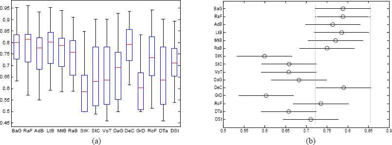
Stage One: Multiple Pairwise Comparison of Combined ELA (FSELA) using AUC
As discussed earlier, DTa and DSt classifiers are used as a base learner but one interesting finding observed in this stage is that DTa outperforms all ELA except StC and VoT (Shows equal performance) in ar3 dataset and DSt outperforms LtB in MW1′ dataset. Moreover, considering the average performance, DTa outperforms StK and GrD, which clearly needs further investigation because in practice ELA always outperform single classifiers for a number of reasons. However, except these cases all ELA outperform single classifiers in all datasets.
Table II shows the ANOVA results for combined ELA with FS, and single classifiers across the AUC result of 17 datasets. The p-value is less than the value of α indicating that the alternate hypothesis is accepted, meaning that, at least two combined Algorithms with FS are significantly different from each other. Figure 2 (a) and (b) show the multiple pairwise comparison results of Stage 1. As RaF achieves high average performance, it statistically significantly outperforms two ELA (StK and GrD). Following that, DeC and BaG statistically significantly outperform four (StK, VoT, GrD and DTa) and two (StK and GrD) algorithms, respectively. The surprising finding observed in this stage is that except DeC no ELA significantly outperforms base learner (DTa) and also LtB doesn’t significantly outperform its base learner (DSt). Moreover, StK and GrD are statistically significantly outperformed by eight and seven ELA, respectively.
5.2. ELA Performance Combined with Feature Selection and Data Balancing
In Figure 3 (a) and (b) and Table VI, the performance comparison of BaG, AdB, RaF, LtB, MtB, RaB, StK, StC, VoT, DaG, DeC, GrD, and RoF combined with both FS and DB are presented. In terms of AUC, again the result of our second experiment suggests that the combined RaF is the most suitable choice for SFP on defect datasets. It demonstrates the highest values in 11 datasets as a winner and 15 results rank as top 3 results out of 17 datasets. Following RaF, RoF (2, 3), MtB (1, 11), DeC (1, 4), LtB (1, 2), DaG (1, 1), BaG (0, 9), AdB (0, 7), and RaB (0, 3) show better performance as a winner and top 3 results, respectively. Considering the average performance after combined implementation with both FS and DB, the results reflect the better performance of combined RaF (0.896), BaG (0.891) and MtB (0.892) with the highest values and outperform the remaining ELA. However, they are closely followed by combined AdB (0.883), DeC (0.881), and RoF (0.880) on software defect datasets. On the other hand, as observed from the experimental results, StK, StC, VoT and GrD appear to perform low when compared with winner and top 3 criteria. In conclusion, based on this performance results (Table II), we can say that, after resolving class imbalance problem with majority datasets, combined RaF consistently demonstrates improved performance, following that BaG and MtB competitively demonstrate good performance. Even though DeC and LtB demonstrate performance improvements, however, they lose their competitiveness in this stage. This means, DeC and LtB are favored by imbalanced nature of the defect dataset (Stage 1) and now (Stage 2) lose their position after resolving class imbalance problem.
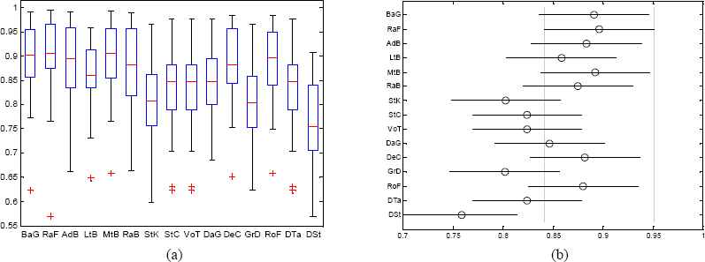
Stage Two: Multiple Pairwise Comparison of Combined ELA (DBFSELA) using AUC
As observed from experimental results, our framework demonstrates the performance of both combined ELA and base learners improves greatly due to resolving class skewness. Moreover, as mentioned in Section V (A), single classifier demonstrates better performance than some of the ELA in some datasets. However, in this stage except considering the average performance StK, and GrD (low performance), and VoT (Shows equal performance), ELA shows better performance. This means, the imbalanced nature of datasets gives advantage. Nevertheless, after resolving the class imbalance problem, ELA becomes powerful, improves classification performance and outperforms base learners. This implies that, ELA are highly biased by class distribution, and the identification of FP module could be compromised by the imbalanced nature of the defect datasets. Thus, with balanced data on selected features, FP modules can be accurately identified as faulty modules so that Software Engineers can dedicate their precious time on the modules that has identified as faulty to resolve the problems before delivering the software product to their customer. This in turn contributes to efficient resource management and produce quality software.
Table III shows the ANOVA results for combined ELA with both FS and DB and single classifiers across the AUC result of 17 datasets. The p-value is less than the value of α indicating that the alternate hypothesis is accepted, this means, at least two combined algorithms with both FS and DB are significantly different from each other. The multiple pairwise comparison results of combined algorithms performance in this stage and their distinctions are clearly depicted in Figures 3 (a) and (b). The surprising findings observed in this stage are only DSt statistically significantly outperformed by seven ELA but the remaining algorithms are not statistically significantly different from each other. The result testifies that how biased class distribution can affect the ELA performance and resolving unfair class distribution on the top of selected features could empower the prediction performance of algorithms contribute for more accurate prediction of faulty module.
5.3. ELA Performance Combined with Feature Selection, Data Balancing and Noise Filtering
In Figure 4 (a) and (b) and Table VII, the performance comparison of BaG, AdB, RaF, LtB, MtB, RaB, StK, StC, VoT, DaG, DeC, GrD, and RoF combined with both FS, DB and NF are given. In terms of AUC indexes, the results of our third experiment show the great performance of combined RaF with both FS, DB and NF. Thus, once again RaF is found to be the most suitable choice for SFP on defect datasets. It demonstrates the highest values in 13 datasets as a winner and 16 results rank as top 3 results out of 17 datasets. Following RaF, AdB (6, 10), RaB (4, 8), DeC (3, 9), MtB (1, 13), RoF (1, 7), BaG (0, 8), LtB (0, 5), and DaG (0, 2) show better performance as a winner and top 3 results, respectively. Considering the average performance after combined implementation with both FS, DB and NF, the results reflect the better performance of combined RaF (0.986), and equal average performance of BaG (0.981), AdB (0.981) and MtB (0.981) of highest values are observed and outperform the remaining ELA. However, they are closely followed by combined DeC (0.980), RoF (0.980), RaB (0.977), LtB (0.968) and DaG (0.955) on software defect datasets. On the other hand, as observed from the experimental results, StK, StC, VoT and GrD again appear to perform low when compared with winner and top 3 criteria. In conclusion, based on this performance results (Table VII), after removing noise instances from the selected features of balanced datasets, combined RaF consistently achieves robust performance. Following that BaG, AdB and MtB competitively show good performance. However, DeC and LtB again lose their competitiveness in this stage. From this, again, we can conclude that, DeC and LtB are favored by imbalanced nature and presence of noise in defect datasets (Stage 1) and now (in Stage 3) lose their position again after resolving class imbalance problem and removing noise instances from defect datasets. With regard to base learners, the same observations are made as Stage 2 including StC (shows equal performance).
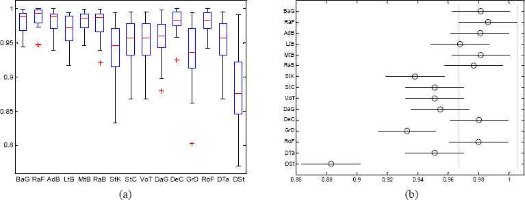
Stage Three: Multiple Pairwise Comparison of Combined ELA (NFDBFSELA) using AUC
In this stage, AdB shows better performance than that in Stage 2. This indications that the presence of noise in the dataset greatly affects AdB ELA. Without noise instances, AdB performs better than with noise instances. Even though the percentage of improvements varies, in general, the performance of all ELA used in this study has revealed great performance improvements. This confirms how powerful is the presence of noise instances in the defect dataset could compromise the ELA performance. It leads us to conclude that combined implementation of noise filtering should be given due attention for more accurately differentiate the FP module from NFP modules.
Table IV shows the ANOVA results for combined ELA and single classifiers with FS, DB and NF, across the AUC result of 17 datasets. Accordingly, the p-value is less than the value of α indicating that the alternate hypothesis is accepted. This means, at least two combined algorithms are significantly different from each other. Here again, RaF ELA statistically significantly outperforms StK, GrD and DSt. In addition to that, StK and GrD are statistically significantly outperformed by eight ELA and except DSt, all other algorithms are not statistically significantly difference from each other.
This implies that removing noise instances gives power to be competitive. One surprising finding observed in this for classifiers performance improvements and makes them stage is that LtB significantly outperforms its base learner (DSt) but no other ELA significantly outperforms its base learner (DTa).
5.4. Multiple Comparison of Three Stages Using Different Performance Metrics
As expected, selecting useful features, resolving class imbalance problem and filtering the presence of noise are found to be useful and improve ELA performance. Our goal here is to investigate whether the combined implementation of ELA with FS, DB and NF can bring additional tangible benefits to the SFP models on defect datasets. In this regard, based on our proposed framework, Sections V (A), (B) and (C) experimental results show the achieved performance improvements. And the more efficiently performed ELA is found to be combined RaF (0. 986) followed by BaG (0.981), AdB (0. 981) and MtB (0. 981) in AUC metrics referring Table VIII. Therefore, this section points out the performance improvement achievements through combined ELA in each stage using average AUC, Accuracy, F-Measure, RMSE and ETT metrics. Accordingly, the combined ELA performance of three different stages and their distinctions are clearly depicted in the Table VIII and Figure 5 (a) to (e).

Multiple Pairwise Comparison of ELA in Each Stage Using Different Metrics
The performance of combined approach with all ELA gives robust results when combining with FS, DB and NF (Stage 3) than the combined implementation in Stage 1 and Stage 2. If we rank the performances of the combined ELA of the different stages, Stage 3 performs the best followed by Stage 2 and finally Stage 1 by Figure 5 (a) and (b). Figure 5 (c) shows great performance improvement after filtering noise instances.
Figure 5 (d) shows prediction errors. It’s surprising to see high prediction error after resolving data skewness. This result can be explained by the fact that even if resolving class distribution problem empowers the prediction power of ELA, it may interpolate some of noise instances. However, noise filtering greatly decreases prediction errors and helps to achieve high accuracy. This is one of the major advantages of combined implementation of FS, DB and NF.
Figure 5 (e) demonstrates average training times of 17 defect datasets with regard to combined algorithms for all three stages. Accordingly, Stage 1 requires less training time than Stage 3, except that in combined RaF and RaB, Stage 1 takes high training time than Stage 3. As Stage 2 has much more instances, it takes more time than Stage 3. In general, DeC requires high training time, following that RaB takes more training time, which clearly indicates that DeC and RaB require more computational cost than other ensemble. Therefore, we can say that other combined algorithms surpass DeC and RaB in terms of training time. The most shortened training time is obtained in LtB, VoT, DaG and base learners. RaF, BaG, AdB, MtB, StK and StC requires reasonable training time as well. These affirms the contribution of three stages based combined preprocessing improves the performance of ELA and reduces computational cost in most of combined ensemble.
ELA performance results for different stages are compared by performing a one-way ANOVA F-test (see Tables IX to XII). Here, the factor of interest considered in ANOVA experiment is the combining strategies (Stage 1, Stage 2 and Stage 3). The null hypothesis for the ANOVA test is that all the group population means (in our case ELA combined with FS, ELA combined with both FS and DB and ELA combined with both FS, DB and NF) are the same, while the alternate hypothesis is that at least one pair of means is different. The significance level for the ANOVA experiment is α = 0.05. Table IX shows the ANOVA results for combined ELA with FS, with both FS and DB and with FS, DB and NF across the average result of 17 datasets. The p-value is less than the value of α indicating that the alternate hypothesis is accepted. That means, the DB and NF solution used in this study has significant contribution to improve the performance of ELA for SFP. The multiple pairwise comparison results of the three stages are shown in Figure 5 (f) to (i). When DB is performed on selected feature (Stage 2), it significantly improves ELA performance compared to the cases where FS is combined alone with ELA (Stage 1). Moreover, when NF is performed on selected features and balanced data (Stage 3), it significantly improves ELA performance compared to the cases where FS is combined alone with ELA (Stage 1) as well as to the cases where FS and DB is combined with ELA (Stage 2).
6. Threat to Validity
There are threats that may have an effect on our experimental results. The proposed prediction models are created without changing the parameter setting except that DTa and DSt algorithms are used with ensemble techniques, which are not default in both cases. Thus, investigations are not made by changing the default parameters setting to see how the variation affects the model performance. In addition to that, as many software metrics are defined in literature. However, we use static code software metrics which are available in selected datasets. Conclusions are drown based on the important features selected using IG, class distribution carried out using SMOTE and noise instances removed using INFFC. In terms of the total instances and number of classes, the datasets may not be good representatives. However, this practice is common among the fault prediction research area.
7. Conclusion and Future Works
This study empirically evaluated the capability of ELA in three stage combined approach in predicting defect prone software modules and compared their prediction performance after combining with FS, after combining with both FS and DB, and after combining with FS, DB and NF in the context of 17 NASA defect datasets. Our objective of using FS, DB and NF was that, by combining those filtering techniques with ELA, we would be able to prune non-relevant features, resolve data skewness and filter noises and then learn an ELA that performs better than from learning on the whole feature set and in imbalanced classes with full of noise instances. Accordingly, the experimental results revealed our combined approach assures performance improvement. On the tested datasets, the highest average result with minimum execution time and minimum prediction error has exhibited when combining ELA with noise filtered balanced class distribution of selected features. As a result, three stages combined ELA is found to be the best approach for SFP. The difference in the performance of the proposed approach of all three stages were statistically tested and confirmed as statistically significant. Therefore, on the top of ELA, using three stage combined approach becomes an added advantage over using only a single classifier. As a result, dealing with the challenges of SFP mentioned in this study, our proposed framework confirms remarkable classification performance which could change SFP practices and lays the pathway to produce quality software products.
For the future work, we plan to employ more preprocessing techniques that help to cleanse the defect datasets and use more defect datasets from different software metrics, and realize how the proposed framework helps to identify more efficient ensemble techniques and improve its classification performance.
References
Cite this article
TY  - JOUR
AU  - Chubato Wondaferaw Yohannese
AU  - Tianrui Li
AU  - Kamal Bashir
PY  - 2018
DA  - 2018/07/04
TI  - A Three-Stage Based Ensemble Learning for Improved Software Fault Prediction: An Empirical Comparative Study
JO  - International Journal of Computational Intelligence Systems
SP  - 1229
EP  - 1247
VL  - 11
IS  - 1
SN  - 1875-6883
UR  - https://doi.org/10.2991/ijcis.11.1.92
DO  - 10.2991/ijcis.11.1.92
ID  - Yohannese2018
ER  -