
Dealing with Missing Data using a Selection Algorithm on Rough Sets
- DOI
- 10.2991/ijcis.11.1.97How to use a DOI?
- Keywords
- Categorical; Imputation; Missing Values; Rough Sets
- Abstract
This paper discusses the so-called missing data problem, i.e. the problem of imputing missing values in information systems. A new algorithm, called the ARSI algorithm, is proposed to address the imputation problem of missing values on categorical databases using the framework of rough set theory. This algorithm can be seen as a refinement of the ROUSTIDA algorithm and combines the approach of a generalized non-symmetric similarity relation with a generalized discernibility matrix to predict the missing values on incomplete information systems. Computational experiments show that the proposed algorithm is as efficient and competitive as other imputation algorithms.
- Copyright
- © 2018, the Authors. Published by Atlantis Press.
- Open Access
- This is an open access article under the CC BY-NC license (http://creativecommons.org/licences/by-nc/4.0/).
1. Introduction
The missing data (henceforth MD) problem is extensively present in real-life databases when working with imperfect information databases, that is, when only vague, incomplete, uncertain and erroneous datasets are available. For example, we may face difficulties when working with surveys due to their frequent lack of information.
Missing data can occur by many factors, such as human errors when filling in the surveys, transcription-process errors, technical bugs in software or corrupted records on the database, among others.
The missing data problem12,1,20 is defined as the absence of relevant data in a information system. Such missing information may be relevant to make data analysis, make decisions or run an algorithm.
In the particular case of this paper, it was motivated by the previous work of the authors on processing information related to armed conflict in Colombia. In that context, there are many incomplete information systems, surveys for instance, so effective methods to take profit of such systems are needed. The authors had used some implementations of LEM2 algorithm to forecast decision variables in some information systems. So, it was interesting to them to apply the rough set theory concepts to the missing value problem.
The quantity of missing data, its pattern (whenever found), the way lost observations occurred, either random or non-randomly, and the kind of data under analysis, are some of the important aspects to take into account to solve this problem. The data under analysis can be symbolic, numerical, textual or any other type.
Three main categories3 of missing data can be established. The first is named Missing Completely at Random (henceforth MCAR) and comprehends cases where no pattern is present in the missing values of the dataset, and all attributes are affected uniformly.
A second category is Missing at Random (henceforth MAR). Unlike MCAR, missing values in this category exhibit certain patterns between their values.
Finally, the third category is Missing not at Random (henceforth MNAR). Missing values in this category follow a certain pattern, but this sort of pattern does not reveal enough information of the value itself.
It is quite difficult to determine the nature of the missing values and classify them in one of these categories, so the techniques used to handle missing values often assume the corresponding information.
Regardless the nature of missing values, the simplest way to deal with missing data examples is just to ignore them and use the rest of the table as the new input. Such action is usually called list deletion. However, this approach may bias the analysis, and it could eventually result in the loss of a significant share of information (when every single case has a missing value). When list deletion is not an option, the simplest solution is to replace voids of missing values with estimations20. The approach that tries to predict those values is called an imputation.
There is no certainty about which is the best algorithm for this purpose or what makes finding imputation algorithms so interesting for research. Algorithms usually exhibit constraints about the kind of data (continuous and discrete data), its distribution, theoretical framework, database size to work with, and the kind of missing values (e.g., MCAR, MAR, and MNAR). Regarding all these factors, imputation algorithms focus on solving imputations for a particular combination of these factors.
Some basic approaches observed in the literature are listed as follows:
- •
Most Common Value and Average Value (henceforth MCV-AV) is a method based on probability theory that replaces missing data values with the most common value of the symbolic attribute, and the average value of numerical attributes. Either the most frequent value or the value with the highest probability can be used, given a certain data distribution (see Refs. 12, 24).
- •
Concept Most Common Value and Concept Average Value (henceforth CMCV-CAV) is a restricted version of MCV-AV based on concepts. A concept is the set of all cases with equal decision value in a decision table (i.e., a database with attributes of condition and attributes of decision). In this method, missing values are replaced with the most common value restricted to the concept, that is, the highest conditional probability attribute-value given by the concept. But when the data is numerical, its missing attributes values are replaced with the average known attribute value restricted to its corresponding concept set (see Refs. 5, 7).
- •
- •
Regression Imputation is a method where the missing observation was imputed using a prediction taken from a multiple regression analysis.
- •
Multiple Imputations for Categorical data is a method that works over a dataset imputing the missing values a fixed number of times using an algorithm to impute single missing values. After running these imputations, the process ends with a fixed number of complete datasets, and yields information about mean, variance and confidence intervals (see Refs. 3, 27).
- •
- •
LEM2 is an algorithm based on LEM algorithm (see Ref. 23). It can handle missing values if we omit examples with unknown attribute values inside the block building step.
- •
The C4.5 algorithm26 represents one of a variety of algorithm based on trees. The algorithm uses a divide-and-conquer approach to create a tree with the data available and its entropy, that is, repeatedly splitting the table by using a similar idea of the concepts.
Other methodologies have been proposed for imputation, based on Neural Networks10,13, Genetic Algorithms13, Bayesian Statistic21,20, Fuzzy Logic17, Clustering21,16,22, Rough Sets6, among others.
The ROUSTIDA algorithm is among the algorithms based on the framework of Rough Sets, which imputes a missing value in a case with a set of similar cases. Then, the algorithm uses a so-called discernibility matrix for handling differences between cases. For a detailed description, we refer the reader to read Ref. 6.
In this paper, a refinement of the ROUSTIDA algorithm is proposed, named ARSI (for Agreements Based on Rough Sets Imputation Algorithm). As indicated by its name, this algorithm is based on the detection of so-called agreements, which are missing data such that similar records in the information system only show one possible value to be imputed. This algorithm uses notions drawn from theory of rough sets, which explains the mention of rough set theory in its name, but the notion of agreement is first presented and used in this paper.
The use of rough set theory to address missing values in information systems is not new. In 1992, Yao and Wong (see Ref. 29) proposed a method based on the theory of rough sets to make decisions from data in a table. This method was extended by Luo and Li (see Ref. 19) to get a way to use incomplete information systems for decision making. Also, Luo et al. (see Ref. 25) developed faster algorithms for these decision procedures. Later, Liu, Liang and Wang (see Ref. 18) extended this method once again for making it possible to make decisions from an incomplete information system that is continuously creating new records from new information. On the other hand, Zhang et al. (see Ref. 30) designed a method to apply MapReduce to compute approximations in parallel on incomplete large-scale information systems.
Rough set theory has been also used to deal with a related problem: The Knowledge Update Problem, which consists of updating the knowledge extracted from an information system that changes along the time. In Ref. 31, the authors develop a rough set rule tree based incremental knowledge acquisition algorithm named RRIA by Rough Set and Rule Tree Based Incremental Knowledge Acquisition Algorithm. This algorithm can learn from a domain data set incrementally, by use of the notion of rule tree. In Ref. 33, the authors also create an incremental algorithm to induce knowledge using the concept of interesting knowledge. In Ref. 32, the author explore the utilization of three matrices (support matrix, accuracy matrix and coverage matrix) for inducing knowledge dynamically.
This paper is structured as follows: In Section 2, the framework of rough sets is briefly introduced. In Section 3, a new algorithm to impute missing values is described. In Section 4, computational experiments with well-known databases are presented. Finally, in Section 5, the discussion is presented and conclusions are given in Section 6.
2. Rough Sets
Rough set theory was proposed by Pawlak as a mathematical framework to conceptualize inaccurate, vague, or uncertain data4,2. Various applications have been developed in Artificial Intelligence using rough sets, like clustering and classification tools1,9,17.
In this paper, a perspective of Rough Sets is used for incomplete information systems where all records are relevant and cannot be ignored, while some attribute values may be unknown. Some basic concepts on this theory are described in order to thoroughly describe the proposed algorithm. We propose Def. 14 and Def. 15. Other definitions and notation can be found in Refs. 1, 8, 9, and 14.
Definition 1.
An information system is a pair (U, A), where U is the set of objects, and A is the set of attributes denoted by A. For every j ∈ A, there is a (possibly partial) function aj : U → Vj. The application of function aj over object x gives its value for attribute j ∈ A where Vj stands for the value set of attribute j. When all the functions aj are total, the system is said to be complete. Otherwise, the system is said to be incomplete.
Definition 2.
An attribute-value pair or just an attribute-value is a pair (j, v), where j ∈ A and v ∈ Vj.
Definition 3.
A missing value is a pair (x, j) such the function aj is not defined at x. When (x, j) is a missing value, we denote it by aj(x) = *.
It is easy to notice that an information system is incomplete if and only if there exists at least one null value or a missing value in some Vj with j ∈ A. Next table is an example of an incomplete information system:
| No. | Sex | Zone | Married | Child |
|---|---|---|---|---|
| 1 | female | 2 | yes | yes |
| 2 | * | * | no | no |
| 3 | male | 3 | * | yes |
| 4 | female | * | yes | no |
| 5 | * | 2 | no | no |
| 6 | male | * | no | no |
Incomplete information system
Since this case’s purpose is to identify the notion of similarity between these objects based on their descriptions, some useful relations are defined as follows:
Definition 4.
Let B ⊆ A. By ∼ TB is denoted the T-tolerance relation module B on U as follows8: Let x, y ∈ U. Then,
According with this tolerance relation module B, it can be established that two objects are indistinguishable if their descriptions based on a set of attributes B are completely included into each other.
For instance, consider the following relations from Table 1. Notice x3 ∼TB x6 with B = {Sex; Zone; Married} and with B = {Sex; Zone; Child} the relation is x4 ∼TB x5 but x4 ≁TA x6.
Another basic concept from this theory is the discernibility matrix, and it serves to indicate which set of attributes makes two objects distinguishable. For incomplete information systems, the following generalization is presented.
Definition 5.
A generalized discernibility matrix MB is a symmetric matrix for a subset of attributes B, x; y ∈ U,
Noted how x ∼TB y implies MB(x, y) = ∅ and so, another useful set was defined, as will be seen later on.
Definition 6.
The I is the set-valued function that assigns a set of objects indistinguishable to x ∈ U,
Definition 7.
The MAS is the set-valued function of all missing attributes for the object x ∈ U,
Definition 8.
The MOS is the set of all objects with at least one missing value on its attribute-value pairs.
Definition 9.
The OMS is the set-valued function over the attribute k ∈ B ⊆ A that outputs all objects with k attribute-value pair missing.
The relation ∼TB described above is certainly symmetric, reflexive and transitive. Now, let’s see a different approach for the concept of similarity seen in Refs. 1, 8.
Definition 10.
Let B ⊆ A. The S-tolerance relation module B (denoted by ∼SB), is defined as follows:
The relation ∼SB, despite being non-symmetric, is reflexive and transitive. It was introduced to handle the absent semantic. Since “x is similar to y” using ∼SB if and only if “the description of x is completely included in the description of y”. For instance, in Table 1, with B = {Sex; Zone; Married}, notice x5 ∼TB x6 but x5 ≁SB x6. It can also seen that x2 ∼SB x5, x2 ∼SB x6, x6 ≁SB x2 and x5 ≁SB x2. Now, the relation ∼SB will be used to define other useful sets.
Definition 11.
The set of objects similar to x,
Definition 12.
The set of objects to which x is similar,
For a deeper discussion of the tolerance relation ∼TB and the non-symmetric relation ∼SB Ref. 1 is recommended.
Definition 13.
Given an attribute value (j, v), a concept based on (j, v) (denoted by C(j, v)), is the set of all objects in X ⊆ U that share the same value v for a given attribute aj,
For instance, concept “yes” of the Child attribute are cases No. 1 and No. 2, and concept “no” will be the set with all rest of the cases.
Definition 14.
Given an attribute aj, and a set X ⊆ U, the existence of an agreement in X on aj is verified, if
Definition 15.
Let x ∈ U and let aj such that aj(x) = *. It is said that aj is ARSI imputable at x, if there is an agreement in set {y ∈ U; x ∼SB y} on aj.
3. ARSI Algorithm
ARSI (Agreements based on Rough Set Imputation) is a deterministic algorithm that imputes MCAR missing values in datasets of categorical data using the framework of the rough set theory presented in Section 2.
The algorithm is presented in Fig. 1. The proposed algorithm is summarized in three main phases, described as follows:
- 1.
Preprocess the information system (line 1).
- 2.
Impute by using agreements (line 2–20).
- 3.
Impute the remaining missing values with an alternative method (e.g., MCV-AV, C4.5) (line 21–25).
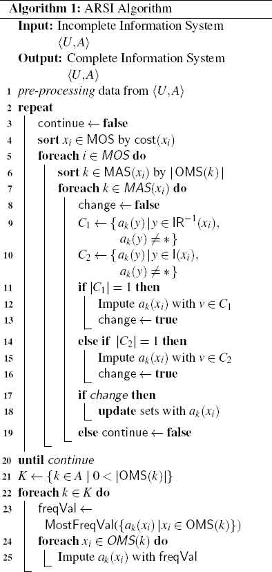
Pseudo-code of the ARSI Algorithm.
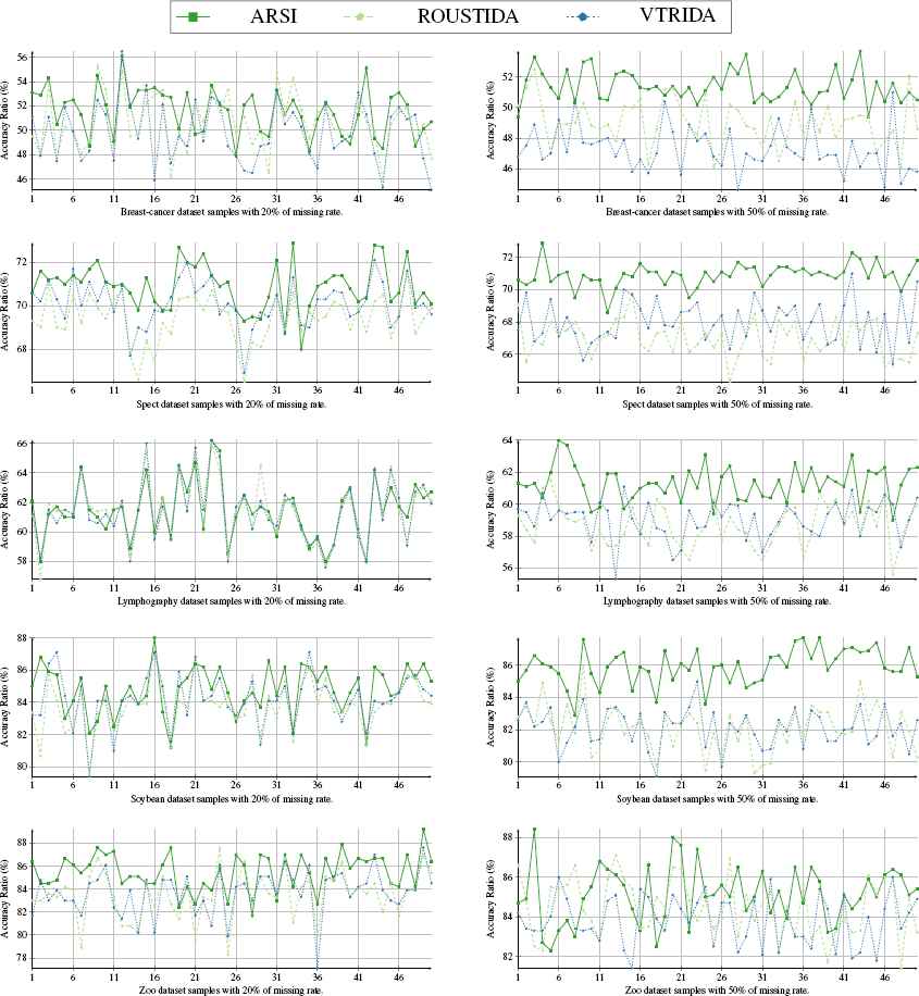
These graphics correspond to the experiments of running all three ARSI, ROUSTIDA and VTRIDA algorithms over all five databases. For each database, 50 tables were obtained with 20% of lost data (graphics on the left) and with 50% of lost data (graphics on the left). The vertical axis in each graphic corresponds to the precision rate (correct imputations vs. number of lost data). The horizontal axis represents the number of sample table.
ARSI is an iterative algorithm to impute “in-place” data, i.e. the imputation is made directly over the same information system.
Prior to the data imputation, a pre-processing routine determines the sets described in Section 2, needed to run the algorithm. These sets are MOS, MAS, OMS, I and R−1. As explained before, it must be taken into account that the contents of these sets is subject to imputation, resulting in a modification of the contents of any of these sets.
In order to simplify the description of the algorithm, the information system U will be referred to as its associated table with n rows and m columns.
Unless stated otherwise, a case x will be defined as a row in the table and instead of referring to the attributes of the case; these will be called the columns of such row. A missing value is a coordinate of row and column in the table and the missing data in a table will be defined as the set of such missing data.
As mentioned before, the ARSI algorithm is iterative. The imputation of a missing datum is always made considering rows first, and then columns. This way, to tell what row should the algorithm complete first, the function cost : U → ℕ × ℕ is used, presented in (3) to make such decision. This function assigns an indicator of the amount of missing information in the row x and of the amount of missing information in its columns. The use of this criterion can be seen in line 4 of the algorithm in Fig. 1.
By virtue of this description, the imputation is made following a lexicographic order. The least cost row is selected and, over said row, its missing values are imputed, one by one, starting with the missing value of the column with more information (lower number of missing data) and finishing with the column with the least information (see lines 5 and 6). If any levelling among columns over the amount of missing information, the algorithm imputes the column on the farthest left.
The imputation of a specific data is described as follows. For the imputation of a missing value in a row x and fix column k, the algorithm verifies the existence of agreements (see Def. 14) in at least one of the sets C1 and C2 defined in (4) and (5), respectively. The sets C1 and C2 were defined based on the tolerance relations S-tolerance and T-tolerance, defined in Def. 10 and Def. 4, respectively.
In lines 11 to 16 it should be clear how the ARSI algorithm has a preference for an agreement in set C1 over an agreement of C2. If any agreement is detected following such preference, the missing value is ARSI imputable (see Def. 15) and the missing value is imputed with the value of the final agreement: line 12 if an agreement was detected by C1 or line 15 if no agreement was detected in C1 and C2 if an agreement was detected.
At the end of an imputation by agreements, the reader must keep in mind that the information system changed and, as a result, the algorithm updates all sets involved in the pre-processing of the table, in a way that the cost function must be updated in every iteration of lines 2 to 19 and takes into account new sets, whenever necessary.
Finally, when there are no more agreements to be imputed by the criteria above mentioned, i.e., when the information system cannot change more in the following iteration, a last stage of the imputation is performed. In such stage, all remaining lost data is imputed using any other of the above-mentioned methods in Section 1. For example, the MCV-AV algorithm was chosen to impute the most frequent value using the MostFreqVal function, lines 21 to 25.
The distribution and the quantity of the missing data in the information system has an important role in the time complexity of the algorithm. If
To finish describing the ARSI algorithm, an example is presented for the information system presented in Table 1.
Example 1.
Consider the information system given in Table 2 from the literature, Ref. 18.
The missing values of this information system are: (O2, 1), (O2, 3), (O3, 4), (O4, 3), (O5, 2), (O5, 3), (O6, 1), (O6, 4), (O8, 2), and (O8, 4).
| A1 | A2 | A3 | A4 | |
|---|---|---|---|---|
| O1 | 3 | 2 | 1 | 0 |
| O2 | * | 2 | * | 0 |
| O3 | 3 | 3 | 1 | * |
| O4 | 2 | 2 | * | 0 |
| O5 | 3 | * | * | 3 |
| O6 | * | 2 | 2 | * |
| O7 | 3 | 2 | 3 | 3 |
| O8 | 2 | * | 2 | * |
Incomplete information system.
Some of the sets computed within the pre-processing stage of the algorithm are shown as follows. Only non-empty sets are shown.
The execution of lines 2 to 19 of the ARSI algorithm described in Fig. 1 for the information system of Table 2 can be summarized in the following description.
When line 4 is run for the first time, the set MAS is sorted by cost function and the result is
This way, following the order in line 5, the first missing datum to be imputed is (O3, 4).
Now, C1 = ∅ and C2 = {3} following their definitions in (4) and (5) respectively. Therefore, the condition of line 11 is not present, but the condition of line 14 is present. That is to say, there is an agreement by set C2 in set {O3, O5} (see Def. 14). Then, the missing datum is imputed (O3, 4) with the value in C2, which is 3.
| A1 | A2 | A3 | A4 | |
|---|---|---|---|---|
| O3 | 3 | 3 | 1 | * |
| O5 | 3 | * | * | 3 |
Similarly, the missing value (O4, 3) is imputed with the value 2 by an agreement in C2. Check that C1 = ∅ and C2 = {2}.
| A1 | A2 | A3 | A4 | |
|---|---|---|---|---|
| O4 | 2 | 2 | * | 0 |
| O2 | * | 2 | * | 0 |
To continue with the order given by set MAS in (6), ARSI tries to impute the missing values (O2, 1) and (O2, 3).
However, it is not possible to find an agreement for these two missing data, since C1 = C2 = {2, 3} and C1 = C2 = {1, 2}, respectively. Without having made any imputation, the next iteration is executed.
Then, the following imputations are considered for the missing data (O5, 2) and (O5, 3), remember that MAS(5) = {A2, A3}. After executing line 7 of algorithm in Fig. 1 becomes evident that C1 = {2} and C2 = {2, 3}. This way, by Def. 15, the missing value (O5, 2) is ARSI imputable to impute with value 2.
| A1 | A2 | A3 | A4 | |
|---|---|---|---|---|
| O5 | 3 | * | * | 3 |
| O7 | 3 | 2 | 3 | 3 |
Following the same criterion, another ARSI imputable agreement is made for (O5, 3). Thus, ARSI imputes with such missing value based on the agreement between O5 and O7.
| A1 | A2 | A3 | A4 | |
|---|---|---|---|---|
| O5 | 3 | 2 | * | 3 |
| O7 | 3 | 2 | 3 | 3 |
After completing iterations (line 2 to line 19), the partial result is Table 4 prior to the imputation with the mean completer (lines 20 to line 25).
| MB | O1 | O2 | O3 | O4 | O5 | O6 | O7 | O8 |
|---|---|---|---|---|---|---|---|---|
| O1 | {} | {} | {A2, A4} | {A1, A3} | {A3, A4} | {A1, A3} | {A3, A4} | {A1, A3} |
| O2 | {} | {} | {A2, A4} | {} | {A4} | {} | {A4} | {} |
| O3 | {A2, A4} | {A2, A4} | {} | {A1, A2, A3, A4} | {A2, A3} | {A1, A2, A3, A4} | {A2, A3} | {A1, A2, A3, A4} |
| O4 | {A1, A3} | {} | {A1, A2, A3, A4} | {} | {A1, A3, A4} | {} | {A1, A3, A4} | {} |
| O5 | {A3, A4} | {A4} | {A2, A3} | {A1, A3, A4} | {} | {A1, A3, A4} | {} | {A1, A3, A4} |
| O6 | {A1, A3} | {} | {A1, A2, A3, A4} | {} | {A1, A3, A4} | {} | {A1, A3, A4} | {} |
| O7 | {A3, A4} | {A4} | {A2, A3} | {A1, A3, A4} | {} | {A1, A3, A4} | {} | {A1, A3, A4} |
| O8 | {A1, A3} | {} | {A1, A2, A3, A4} | {} | {A1, A3, A4} | {} | {A1, A3, A4} | {} |
Generalized discernibility matrix of the information system of Table 2.
| A1 | A2 | A3 | A4 | |
|---|---|---|---|---|
| O1 | 3 | 2 | 1 | 0 |
| O2 | * | 2 | * | 0 |
| O3 | 3 | 3 | 1 | 3 |
| O4 | 2 | 2 | 0 | 0 |
| O5 | 3 | 2 | 3 | 3 |
| O6 | 2 | 2 | 2 | 0 |
| O7 | 3 | 2 | 3 | 3 |
| O8 | 2 | 2 | 2 | 0 |
ARSI imputation of the information system in Table 2 before using the mean completer method.
A comparison can be made at this point by considering the result after using the ROUSTIDA algorithm on the same database. The ROUSTIDA outputs18 the imputation shown in Table 5. As we can notice from this table, ARSI is able to impute more missing values than ROUSTIDA. In Section 4 we will see other comparisons.
| A1 | A2 | A3 | A4 | |
|---|---|---|---|---|
| O1 | 3 | 2 | 1 | 0 |
| O2 | * | 2 | * | 0 |
| O3 | 3 | 3 | 1 | 3 |
| O4 | 2 | 2 | 2 | 0 |
| O5 | 3 | * | * | 3 |
| O6 | * | 2 | 2 | * |
| O7 | 3 | 2 | 3 | 3 |
| O8 | 2 | 2 | 2 | 0 |
ROUSTIDA imputation of the information system in Table 2 before using a mean completer approach.
Finally, the mean completer is used to complete the imputation of the missing values. Remember that in this step any other algorithm could be used for this kind of imputation. The final result of the imputation of the ARSI algorithm for Table 2 is shown in Table 6.
| A1 | A2 | A3 | A4 | |
|---|---|---|---|---|
| O1 | 3 | 2 | 1 | 0 |
| O2 | 3 | 2 | 2 | 0 |
| O3 | 3 | 3 | 1 | 3 |
| O4 | 2 | 2 | 0 | 0 |
| O5 | 3 | 2 | 3 | 3 |
| O6 | 2 | 2 | 2 | 0 |
| O7 | 3 | 2 | 3 | 3 |
| O8 | 2 | 2 | 2 | 0 |
The same information system after using the ARSI algorithm to impute missing data values using a mean completer approach.
4. Experimental Results
The performance of the ARSI algorithm was evaluated by running the following experiment.
We chose five representative categorical datasets from UCI Machine Learning Repository15: Breast Cancer, Soybean, Lymphography, Spect, and Zoo dataset. We compared the performance of the ARSI algorithm against other two algorithms for imputation in rough set theory, the ROUSTIDA6 and VTRIDA14 algorithm. The ARSI algorithm is presented as an refinement of the ROUSTIDA algorithm in Section 3 whereas the VTRIDA algorithm shows to be better than ROUSTIDA in Ref. 14.
All results of this experiment, along with the implementations of ARSI, ROUSTIDA and VTRIDA algorithms are available to the public in the repository http://github.com/jonaprieto/imputation. The experiments were conducted in Mathematica software and implemented the ARSI, ROUSTIDA, and VTRIDA algorithms using the Wolfram Language programming. This way, the reader can modify this experiment to remove a different percentage of missing data, use other databases or modify the algorithms. Other results available in the referenced repository are not shown here due to the greater extension these would add to this document. These experiments were made with missing data percentages of 15%, 25%, 35%, and 45%.
In Table 7 a summary of the characteristics of the datasets is presented. For each dataset, fifty samples were randomly generated with a fixed percentage of missing values without any pattern. Then, all missing values were MCAR missing data type.
| No. | Dataset | Instances | Attributes |
|---|---|---|---|
| 1 | Breast Cancer | 277 | 10 |
| 2 | Lymphography | 148 | 19 |
| 3 | Soybean | 63 | 36 |
| 4 | Spect | 267 | 23 |
| 5 | Zoo | 101 | 17 |
List of test datasets
Shares of 5%, 10%, 20%, 30%, 40% and 50% of values were randomly removed from each dataset sample. In this process, each dataset sample was obtained avoiding any empty row or column. Each dataset was examined in a way that guaranteed there were no empty rows or columns. For this, the following function*, implemented in Mathematica, was used.
MakeArrange[{n_, m_}, p_] := Module[
{cand, base}
base =
PadLeft[
ConstantArray[1, Round[n*m*p]]
, n*m
];
While[(
cand =
ArrayReshape[
RandomSample@base
, {n, m}
];
Max[Total[cand]] > n - 2
| | Max[Total /@ cand] > m - 2)];
Return[Position[cand, 1]];
];
The function’s arguments are the following: the size of table of the information system, n × m and a percentage, p, for the amount of missing data requested. The expected outcome using this function is a list of positions (row, column), that shall be erased in the dataset to yield the lost values, with the required percentage of loss.
This way, the experiment comprised 4500 datasets to run the validation over (3) algorithms, (6) missing rates, (5) datasets, (50) samples per each dataset.
In order to measure the accuracy of each algorithm, each output of the algorithm was compared with the original dataset. Information about mean, variance, maximum and minimum accuracy, as well as the confidence interval was collected in Table 8 and Table 9.
| Dataset | 5.0% | 10.0% | 20.0% | |||||||
|---|---|---|---|---|---|---|---|---|---|---|
| ARSI | ROUSTIDA | VTRIDA | ARSI | ROUSTIDA | VTRIDA | ARSI | ROUSTIDA | VTRIDA | ||
| B. Cancer | Min | 42.4 | 42.4 | 40.8 | 45.8 | 46.2 | 43.8 | 47.9 | 45.9 | 45.1 |
| Max | 61.6 | 61.6 | 60.8 | 57.4 | 58.2 | 57.8 | 56.1 | 55.3 | 56.5 | |
| Mean | 52.1 | 52.1 | 51.7 | 51.7 | 51.6 | 50.9 | 51.6 | 50.6 | 49.8 | |
| Int. | [50.7 53.6] | [50.8 53.4] | [50.3 53.1] | [51.0 52.5] | [50.8 52.4] | [50.1 51.7] | [51.0 52.1] | [50.0 51.3] | [49.1 50.5] | |
| Spect | Min | 65.0 | 64.6 | 65.0 | 65.8 | 66.1 | 66.6 | 68.0 | 66.5 | 66.9 |
| Max | 75.2 | 73.8 | 75.5 | 73.6 | 72.9 | 73.8 | 72.9 | 71.5 | 72.1 | |
| Mean | 70.2 | 69.6 | 70.2 | 70.2 | 69.4 | 70.1 | 70.9 | 69.4 | 70.1 | |
| Int. | [69.5 70.8] | [68.9 70.2] | [69.5 70.9] | [69.8 70.6] | [68.9 69.8] | [69.6 70.5] | [70.6 71.2] | [69.1 69.7] | [69.8 70.4] | |
| Lymph. | Min | 52.6 | 52.6 | 52.6 | 55.3 | 55.3 | 55.3 | 58.0 | 56.8 | 57.6 |
| Max | 73.7 | 73.7 | 73.7 | 68.8 | 68.8 | 68.8 | 66.2 | 66.0 | 66.2 | |
| Mean | 61.4 | 61.4 | 61.4 | 61.5 | 61.5 | 61.6 | 61.5 | 61.4 | 61.4 | |
| Int. | [60.1 62.7] | [60.1 62.7] | [60.1 62.7] | [60.7 62.3] | [60.7 62.3] | [60.8 62.4] | [60.9 62.0] | [60.8 62.0] | [60.8 62.0] | |
| Soybean | Min | 78.2 | 77.3 | 77.3 | 80.9 | 80.9 | 80.0 | 81.2 | 79.6 | 79.4 |
| Max | 93.6 | 93.6 | 93.6 | 89.5 | 89.5 | 89.5 | 88.0 | 87.3 | 87.1 | |
| Mean | 86.1 | 86.0 | 86.1 | 85.6 | 85.3 | 85.5 | 84.8 | 83.9 | 84.2 | |
| Int. | [85.1 87.1] | [85.0 87.0] | [85.2 87.1] | [85.0 86.1] | [84.7 85.9] | [84.9 86.2] | [84.4 85.2] | [83.4 84.3] | [83.8 84.7] | |
| Zoo | Min | 72.8 | 72.8 | 75.3 | 77.2 | 74.7 | 75.3 | 81.7 | 78.3 | 77.1 |
| Max | 90.1 | 88.9 | 91.4 | 88.3 | 87.0 | 87.7 | 89.2 | 87.6 | 87.6 | |
| Mean | 82.5 | 80.9 | 82.0 | 84.1 | 82.5 | 83.1 | 85.5 | 83.5 | 83.7 | |
| Int. | [81.5 83.5] | [79.8 82.0] | [81.0 83.1] | [83.3 84.9] | [81.6 83.3] | [82.2 84.0] | [85.0 86.0] | [82.9 84.1] | [83.1 84.3] | |
Results of the experiments when databases of 5%, 10% and 20% of missing data. The results in bold show when ARSI got the best absolute result.
| Dataset | 30.0% | 40.0% | 50.0% | |||||||
|---|---|---|---|---|---|---|---|---|---|---|
| ARSI | ROUSTIDA | VTRIDA | ARSI | ROUSTIDA | VTRIDA | ARSI | ROUSTIDA | VTRIDA | ||
| B. Cancer | Min | 47.9 | 46.5 | 44.0 | 48.8 | 45.9 | 44.3 | 49.4 | 46.1 | 44.6 |
| Max | 54.5 | 53.9 | 52.9 | 53.9 | 52.5 | 51.0 | 53.7 | 52.5 | 51.0 | |
| Mean | 51.2 | 49.9 | 48.5 | 51.5 | 49.3 | 48.0 | 51.4 | 49.0 | 47.3 | |
| Int. | [50.7 51.7] | [49.4 50.4] | [48.1 49.0] | [51.1 51.9] | [48.9 49.8] | [47.6 48.4] | [51.1 51.7] | [48.6 49.5] | [46.9 47.7] | |
| Spect | Min | 69.7 | 66.8 | 68.0 | 69.4 | 66.0 | 66.7 | 68.6 | 64.3 | 65.4 |
| Max | 73.4 | 71.7 | 72.7 | 74.9 | 70.3 | 72.1 | 72.9 | 69.8 | 71.0 | |
| Mean | 71.8 | 69.1 | 70.2 | 71.9 | 68.3 | 69.1 | 70.9 | 67.0 | 68.0 | |
| Int. | [71.6 72.1] | [68.7 69.4] | [69.8 70.5] | [71.6 72.2] | [68.0 68.6] | [68.8 69.5] | [70.7 71.1] | [66.7 67.3] | [67.7 68.4] | |
| Lymph. | Min | 57.7 | 56.3 | 56.4 | 57.5 | 56.5 | 57.6 | 59.0 | 55.6 | 55.3 |
| Max | 64.0 | 63.8 | 64.0 | 63.4 | 62.2 | 63.3 | 64.0 | 61.5 | 61.1 | |
| Mean | 61.2 | 60.6 | 60.7 | 61.1 | 59.4 | 59.7 | 61.3 | 58.7 | 59.0 | |
| Int. | [60.7 61.7] | [60.1 61.1] | [60.3 61.2] | [60.8 61.5] | [59.0 59.8] | [59.3 60.1] | [61.0 61.6] | [58.3 59.0] | [58.7 59.4] | |
| Soybean | Min | 82.2 | 79.8 | 79.2 | 83.7 | 79.0 | 78.7 | 82.9 | 79.3 | 79.1 |
| Max | 87.5 | 85.3 | 86.0 | 89.2 | 85.7 | 86.1 | 87.7 | 86.0 | 85.0 | |
| Mean | 84.4 | 82.8 | 82.9 | 85.7 | 82.4 | 82.5 | 85.9 | 82.1 | 82.1 | |
| Int. | [84.1 84.7] | [82.4 83.1] | [82.5 83.3] | [85.4 86.0] | [81.9 82.8] | [82.1 83.0] | [85.6 86.2] | [81.7 82.5] | [81.8 82.5] | |
| Zoo | Min | 83.9 | 81.0 | 80.2 | 81.6 | 80.7 | 79.9 | 82.3 | 81.4 | 81.4 |
| Max | 89.7 | 88.5 | 86.8 | 89.2 | 89.2 | 86.8 | 88.4 | 87.1 | 86.0 | |
| Mean | 87.1 | 84.7 | 84.2 | 86.0 | 84.8 | 84.0 | 85.1 | 84.5 | 83.8 | |
| Int. | [86.8 87.5] | [84.3 85.1] | [83.7 84.6] | [85.5 86.5] | [84.4 85.2] | [83.6 84.5] | [84.7 85.5] | [84.1 84.9] | [83.5 84.2] | |
Results of the experiments when databases had 30%, 40% and 50% of missing data. The results in bold show when ARSI got the best absolute result.
In these tables, it becomes evident that in the cases where the lost data is less than or equal to 10%, the ARSI algorithm did not show a significant difference in comparison with the accuracy of other algorithms’ imputations. Even in some cases ARSI’s imputation accuracy was equal to the accuracy of the ROUSTIDA or VTRIDA algorithm. Without reaching the best results nor the lowest accuracy of imputation, ARSI with a low missing data percentage did not clearly show its performance and improvements in comparison with its competitors in imputation.
However, when the loss percentage was increasing, ARSI got the best results in imputation. The results in bold in the aforementioned tables refer to the occasion when ARSI was the best at accuracy in imputation).
Now, based on the confidence interval of the three algorithms in each database and with a fixed percentage of lost data, we observed that in 95% of the experiments conducted, the imputation accuracy was always higher using ARSI than using ROUSTIDA or VTRIDA (see the accuracy value of each confidence interval’s lowest extreme of the ARSI results compared to the confidence intervals’ lowest extremes of the imputations with other algorithms).
To have a better view of the algorithms’ effectiveness and of the comments above, the graphics of the results for each algorithm are shown in Fig. 4, as well as each database when the percentage of lost values was 20% and 50%.
From these graphics ARSI proved to be a competitive algorithm. In each graphic, ARSI algorithm imputes with the higher precision most of the times as compared to the imputations made by the other algorithms, ROUSTIDA and VTRIDA. For example, it is clear that ARSI is significantly superior to ROUSTIDA and VTRIDA in all the examples, for the dataset Spect with 50% of lost data, SoyBean with 50% of lost data and Breast Cancer with 50% of lost data. In the other graphics, while ARSI’s accuracy is not indisputably the best, the number of times that it had the lesser accuracy is significantly lower than its competitors (see for example this behavior in the graphic for Lymphography with 50% of MD, Zoo with 20% of MD, Zoo with 50% of MD and Spect with 20% of MD).
The accuracy and results of the ARSI algorithm were observed to be significantly better than its competitors as the percentage of lost data increases. This behavior can be seen in Fig. 4, when said percentage was increased from 20% to 50% of lost data; this confirms what was stated above. ARSI imputed clearly better as the percentage of lost data got higher.
5. Discussion
ARSI is an algorithm based on rough set theory. The computation involved in the core imputation process of ARSI demands a high amount of computing resources and, as happens with other algorithms based on similar ideas on Rough Sets, it can cause a high cost of memory for large databases as imputation is reaching its end.
Considering this, MB, I, MAS, R−1 and MOS sets were precomputed in order to reduce overhead in computation while efficiently performing update routines in running time as other details in the implementation. ARSI is known to need further improvements to scale for running on large databases, while on the other hand, experimental results proved that ARSI algorithm, on most cases, performed better or equal than its competitors ROUSTIDA and VTRIDA algorithms.
However, when the experiments showed that ARSI imputed better when the percentage of lost data increased. It can be inferred that, in the core of the algorithm, the agreements allow the imputation to be made. The bigger the quantity of lost information, the more frequent such agreements can be found, since these agreements are produced when descriptions of certain objects are contained in other descriptions (see the Def. 14). When an object’s description has more lost data there is more chance of finding other objects with similar descriptions under the same similarity relations (see Def. 10 and Def. 4). In other regards, since ARSI’s efectivity and behavior is better, as the percentage of missing data increases it has to disappear eventually.
When the information system’s information becomes insufficient to generate agreements, the algorithm’s core uses the alternative imputation method to complete the imputation. Then, this last step plays an essential role when the percentage of lost data is significantly low and when it is high.
It was seen that, similar to ROUSTIDA or VTRIDA, this last step of ARSI is critical in the performance of the algorithm. A possible improvement for this step, would be exploring another method instead of MCV-AV like multiple imputations27, classification as imputation or using induction rules (see for instance Ref. 16 for a treatment of imputing missing values using classifiers based on decision trees’ techniques).
6. Conclusions
In this paper, the ARSI algorithm was proposed in order to impute missing values in categorical databases using the framework of rough set theory. The core of the ARSI algorithm is based on a similarity relation, generalized discernibility matrix, and a selection criterion. Through computational experiments, the ARSI algorithm was confirmed to be as efficient and competitive as other imputation algorithms based on rough sets theory. Moreover, ARSI behaved as the best algorithm in the experiments when the missing data rate were increasing.
The ARSI algorithm still need improvements in some computational aspects like memory usage. Additionally, it could be improved by replacing the method that imputes in the last part of the algorithm (mean completer) with another imputation algorithm.
Lastly, ARSI can be extended in order to handle another kind of missing data values rather than just categorical data with MCAR database condition. We point out these improvements for future work.
Footnotes
Based on the function provided on http://goo.gl/5O7jhs
References
Cite this article
TY  - JOUR
AU  - Jonathan Prieto-Cubides
AU  - Camilo Argoty
PY  - 2018
DA  - 2018/07/11
TI  - Dealing with Missing Data using a Selection Algorithm on Rough Sets
JO  - International Journal of Computational Intelligence Systems
SP  - 1307
EP  - 1321
VL  - 11
IS  - 1
SN  - 1875-6883
UR  - https://doi.org/10.2991/ijcis.11.1.97
DO  - 10.2991/ijcis.11.1.97
ID  - Prieto-Cubides2018
ER  -