
An Integrated Algorithm of CCPP Task for Autonomous Mobile Robot under Special Missions
- DOI
- 10.2991/ijcis.11.1.100How to use a DOI?
- Keywords
- Autonomous mobile robot; Complete coverage path planning (CCPP); Integrated algorithm; Chaotic path planner; Cellular decomposition approach; The Standard map
- Abstract
Due to the difficult problem of avoiding obstacles to achieve the complete coverage path planning (CCPP) for special missions, this paper introduces a novel integrated algorithm of CCPP for autonomous mobile robot under an obstacles-included environment. The algorithm combines cellular decomposition approach and the Standard map together for designing. The cellular decomposition approach is used to simplify the given workplace into smaller sub-regions for coverage via a chaotic path planner. The planner is constructed based on the chaotic Standard map at full mapping and produces the needed trajectories inside each decomposed sub-region. The simulation results verify the effectiveness of the designed method.
- Copyright
- © 2018, the Authors. Published by Atlantis Press.
- Open Access
- This is an open access article under the CC BY-NC license (http://creativecommons.org/licences/by-nc/4.0/).
1. Introduction
With wide applications of the intelligent robot in domains, for example, the vacuum cleaning1, harvesting2, lawn mowing3, underwater sources exploring4, unmanned aerial vehicles (UAV)5,6,7 and so on, one of the core technologies, complete coverage path planning (CCPP), has received extensive attentions. CCPP is the task of determining a path that passes over all points of an area or volume of interest while avoiding obstacles8. In the above circumstances, only the complete coverage of the entire terrain is needed. While for some special missions, especially in the circumstances for military applications, such as the surveillance of terrains9, the terrain exploration for searching10, demining11, and patrolling12, high unpredictability or randomness for the robot trajectories, as well as fast scanning of the workplace area are strongly required.
In 2001, Nakamura and Sekiguchi proposed a strategy to solve the above mentioned problems based on chaotic systems13. In that work, the chaotic behavior of the Arnold dynamical system was imparted to the mobile robot’s motion control. Since then a great number of relative research works in the field of autonomous mobile robots have been presented, because the chaotic motion guarantees the scanning of the whole workspace without a terrain map or motion plan and can obtain unpredictable trajectories. The main characteristics of the chaotic systems are the topological transitivity and the sensitive dependence on initial conditions14. Due to topological transitivity, the chaotic mobile robot is guaranteed to patrol the whole surveillance region completely without repetitions. The sensitive dependence on initial conditions is a desirable characteristic for patrol robots, since the trajectory produced by the chaotic mobile robot is unpredictable or random15,16,17. Chaotic system is very different from the random signal. The chaotic motion is based on determinism, which in the case of mobile robots is an advantage. This happens because the behavior of a robot can be predicted in advance by the system designer.
The purpose of using chaotic systems in autonomous robots is realized by designing the chaotic path planner, which ensure chaotic motion. The trajectories produced by it are used to guide autonomous robots for exploration of a terrain for vigilance. In the literature, Lorenz dynamical system18,19, Standard or Taylor-Chirikov map 9,10,21, Chua circuit 22, Logistic map23, and double-scroll systems15,24,25 are some of the chaotic systems which have been commonly used for this purpose. We also constructed two chaotic motion path planners26,27, which were improved by arcsine or arccosine transformations, based on the Logistic map and Chebychev map, respectively, for an autonomous mobile robot to cover an unknown terrain completely, unpredictably, and evenly.
In the workplace without obstacles, the trajectories produced by the chaotic path planner can demonstrate the same performance as the original chaotic system, and meet the requirements of special missions. But it is difficult to design an obstacles avoiding strategy in an obstacles-included environment using the chaotic path planner while maintaining the chaotic characteristics of the coverage trajectories unchanged. Most of the researches now use the mirror mapping method to avoid obstacles for the chaotic mobile robot13,28,29,30. It really works when the distances between two adjacent iterative points produced by the chaotic system are very short, because it only requires the measurement of the local normal of the boundaries of workspace or obstacles when the robot comes close to them. But to the systems that the distances are very large, the method is not applicable because of the frequently used of the mirror mapping almost at each iterative step. So the trajectories produced by mirror mapping method will occupy larger part of the total coverage trajectories which can influence the chaotic characteristics of the coverage trajectories. Furthermore, it has to judge whether the produced trajectory will collide with the obstacles or not in each planning step, which can increase computation complex of the method and decrease the planning efficiency.
This paper introduces an integrated algorithm to solve the above problem based on the chaotic Standard map and cellular decomposition approach. The Standard map, or called Taylor-Chirikov, is a well known two-dimensional mapping 31. Martins-Filho and Macau9 proposed an ingenious path-planning mechanism where the sequence of intermediary goal positions were obtained using the map. We also proposed a fusion iterations strategy based on the map to generate a chaotic path planner of autonomous mobile robot for surveillance missions32,33. The Standard map is easy to be controlled for having a single parameter K which determines its state. Its two variables (xn,yn) can be directly mapped to the robot’s position or coordinates in the workplace. Furthermore it has the better coverage property in running region for its full mapping characteristics at the chaotic state when K ≥ 8. So we use the chaotic Standard map at K = 8 to construct the chaotic path planner, and combine the cellular decomposition method to achieve the CCPP task under special missions.
The cellular decomposition method simplifies the complex coverage task into some simple sub-regions or cells for covering. Choset conjectured that most complete algorithms used an exact cellular decomposition of the free space, either explicitly or implicitly, to achieve coverage34. It partitions the given environment into several smaller sub-regions, and each sub-region is covered by the robot in a prescribed manner. Once each sub-region has been covered, the overall coverage task is realized.
In this research, the given workplace including obstacles has been divided into some cells, then the rectangular feasible sub-regions are formed by them based on a merging strategy. The chaotic path planner constructed by the Standard map realizes the coverage task in decomposed sub-regions. The size of each sub-region should be in a rectangular shape to correspond to the running domain of the Standard map. The attractor characteristics of the chaotic path planner eliminates the detection of obstacles and boundaries of the workplace when the robot is covering inside a sub-region. After achieving the coverage task in one sub-region, the robot goes to another one by a safety zone, which is established to design the transition procedure between two adjacent sub-regions to avoid obstacles based on the attractor characteristics also. Avoidance of obstacles only occur during transition procedure and needs two steps at most to achieve one transition. Compared with mirror mapping method, the designed obstacles’ avoidance method is very simple and efficient. The transition trajectories occupy little part of the whole coverage trajectories and have little effect to the chaotic characteristics of them. So under an obstacles-included environment, the constructed chaotic path planner can produce the coverage trajectories to achieve the CCPP task for special missions, with completeness, unpredictability, evenness and safety.
Some work above has been discussed in [33]. This paper further put forward the following new ideas:
- (i)
A systematic approach of merging strategy has been formed for constructing the rectangular iterative sub-regions. It simplifies the merging procedure and can be easily achieved by computer;
- (ii)
The attracting property of the chaotic Standard map is used for designing the transition procedure to facilitate the coverage procedure and improve the coverage efficiency.
- (iii)
The safe-zone is established to avoid the obstacle based on the attracting property of the chaotic Standard map. Only after two steps at most, the transition procedure can be achieved safely and conveniently.
The rest of the paper is organized as follows. The basic characteristics of the Standard map in the chaotic state are presented in Section 2. Section 3 constructs the chaotic path planner based on the Standard map at the fulling mapping state. The detailed designing procedure of the integrated algorithm based on cellular decomposition approach and the chaotic Standard map is described in Section 4. Section 5 illustrates a case to verify the designed algorithm. The last section outlines the conclusions and future work.
2. Characteristics of the Standard Map
The Standard map, or the Taylor-Chirikov, is a two-dimensional areas preserving dynamical system 35,36. Area-preserving mappings give rise to incredibly rich dynamics and mathematics 37,38. The researchers commonly use the following discrete formula of the Standard map to model the chaotic path planner for an autonomous mobile robot:
2.1. Bifurcation diagrams
Parameter K controls the dynamic properties of the Standard map. As it increases, the map evolves from double-periodic bifurcation to the chaotic state. Fig. 1 illustrates the bifurcation diagrams of the two variables with successive changing of the parameter K, respectively. When K is greater than a certain value, the iterative values of xn and yn are full of the entire running domain, namely the system owns the completeness.
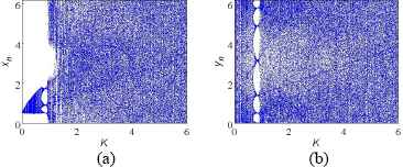
Bifurcation diagram (a) xn vs. K and (b) yn vs. K.
2.2. Phase space
Bifurcation diagrams of Fig. 1 can not distinguish the boundaries clearly among different states of the system due to resolution of the picture, so the method of phase space is used to further analyze the state changing. Fig. 2 shows the phase space of the map for parameter K with varying values. As K increases, the trajectories fill a larger region of the phase space. As K = 5, seen in Fig. 2(c), only a small two blank windows are left. In Fig. 2(d), for K = 8, one has an impression that chaos is complete, and the system is at a full mapping state in phase space. So parameter K can assume an integer value equal or greater than 8 for the system to obtain a complete covering trajectories in its iterative region. It has a good distribution feature and is suitable for achieving the coverage mission.

Phase space of the the Standard map vs. K (for x0 =0.5, y0=0.5, n=10,000) (a) K=1, (b) K=4, (c) K=5 and (d) K=8.
2.3. The largest Lyapunov exponent
The largest Lyapunov exponent (LLE) is an important evaluation index of the chaotic state for a system. If LLE > 0, the system can be assured to be chaotic39. And the greater the exponent is, the better the chaotic performance the system shows. Using 5,000 sampled time sequences of xn computed by formula (1), the LLE spectrum, shown in figure 3, is calculated based on the reconstructed attractor method40.
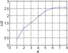
Spectrum of LLE with parameter K
The picture shows that LLE is always greater than 0 when K takes the positive integer. So the system keeps at the chaotic state owning these values, and has the maximum LLE as K=8, which is about 2.6. The system with this value has the best chaotic characteristics and is at the full mapping state, which is shown in Fig. 2 (d). It is beneficial for the robot to produce the random and coverage trajectories. So the following map is used to achieve the CCPP task for the robot:
2.4. Distribution characteristics of the coverage trajectories
The variables (xn, yn) produced by Eq. (2) can be used as the planned intermediary waypoint of CCPP for autonomous mobile robot. Connection of all the sub-goals according to the produced-order sequence constitute the coverage trajectories for robot to track. The planned results are shown in Fig. 4 and Fig. 5.
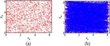
Planned results of the coverage path planning at n=2,000 (a) planned sub-goals and (b) planned coverage trajectories.
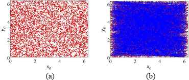
Planned results of the coverage path planning at n=5,000 (a) planned sub-goals and (b) planned coverage trajectories.
From the above analysis, one can conclude that the planned sub-goals (xn, yn) and coverage trajectories produced by the Standard map at K = 8, have a very good uniformly distribution and can guarantee the complete coverage. It can meet the requirements, e.g., completeness, evenness, and unpredictability for special missions of CCPP task.
3. The Chaotic Path Planner
To cover a blank region of rectangular size, the trajectories produced by Eq. (2) can be used as the coverage path of CCPP task for autonomous mobile robot. Fig. 4 and Fig. 5 show that the operating range of (xn, yn) is restricted in a rectangular scope [0 2π 0 2π]. By affine transformation based on Eq. (2), the running domain of (xn, yn) can be mapped to a rectangular region of any size from the original one:
The designed chaotic path planner has attractor characteristics. Whether the initial point (x0, y0) is within the iterative region or not, the successive iterative values (x1~xn) and ( y1~yn) are all bounded between (0,2π) because of the modular calculation by 2π in the original Standard map. So its iterative region also can be called as attracting area. After affine transformation, the attracting area can be mapped to a rectangle with any shape.
Suppose there is a workplace with size 10×10. Then the rectangular area [0 10 0 10] is its attracting region. The affine parameters [a b c d] of the constructed chaotic path planner is [0 0 10/2π 10/2π]. It produces the coverage trajectories based on the given (x0, y0) and Eq. (3). Fig. 6 illustrates the attractor characteristics of the chaotic path planner based on the planned coverage trajectories, where the circles “o” express the initial point (x0, y0), the small little points mark other iterative values, and blue lines show the planned coverage trajectories.
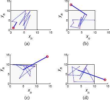
Attractor characteristics at n=10 (a) (x0, y0)=(1,1), (b) (x0, y0)=(1,13), (c) (x0, y0)=(14,14) and (d) (x0, y0)=(14,2).
In Fig. 6.(a), (x0, y0) locates inside the workplace. No matter how many times the system iterates, the iterative values (xn, yn) always lie in the workplace, and the robot can’t collide with the boundaries of the workplace. So we needn’t have to design the boundaries’ avoidance method for the robot when it runs inside its attracting region. In Fig. 6.(b)~(d), though (x0, y0) locates outside the workplace, only after one iterative step, the robot goes into the attracting area [0 10 0 10]. Using the property, we can design the transiting strategy to achieve the transition between two adjacent sub-areas.
4. Integrated Algorithm Designing
In a rectangular workplace including obstacles, cellular decomposition method is used to partition the workplace and some feasible iterative sub-regions are formed. When the autonomous mobile robot completes the coverage task by the chaotic path planner in each iterative sub-region in turn, the whole CCPP task realizes. The integrated algorithm includes partition of workplace, construction of the iterative sub-regions, establishment of the safety zones and the transition procedure design, formation of the coverage connected-path, and the coverage procedure to achieve the CCPP task. All the partitioned and constructed sub-regions must be in a rectangular size to correspond to the shape of running domain or attracting region of the chaotic path planner.
4.1 Partition of the workplace
In an enclosed rectangular workplace including obstacles, the connected free areas without obstacles are partitioned into some smaller grids, labeled as Sx, along the boundaries of obstacles and workplace, and the subscript x expresses the symbol of each Sx. Some parallel vertical and horizontal straight lines are used to segment the workplace. They extend to both sides along the obstacles’ boundaries until meet the borders of workplace or the boundaries of other obstacles. Then the small adjacent rectangles Sx are obtained from the crossing areas which are produced by the segment lines in feasible areas. The number of Sx is related to the obstacles’ number and positions in workplace.
4.2 Construction of the iterative sub-regions
In order to reduce the transition times, the number of the needed coverage sub-regions is the less, the better. Here we define a iterative sub-region, labeled as SI_x, to merge the partitioned grids Sx. There are many methods that can be used. In our previous work 33, the corner rectangles were defined to design the method. Here, another simpler merge algorithm is designed. First select a merging direction and a group of parallel lines based on it. The merging direction can be chosen from the followed ones, namely from top to bottom, bottom to top, left to right or right to left. The parallel lines include the above partition segment lines and the border lines of workplace. Then a rectangular iterative sub-region SI_x can be constructed by all Sx between two adjacent parallel lines. The final number of SI_x is same as other methods obtained and has the least value. The detailed strategy is described in Algorithm 1.
The functions contained in Algorithm 1 are introduced as follows:
- •
Direction_select (i): The function is to select a merging direction. There are four directions for being selected:
i=1, Direction_select (1)=1, from top to bottom;
i=2, Direction_select (2)=2, from bottom to top;
i=3, Direction_select (3)=3, from left to right;
i=4, Direction_select (4)=4, from right to left.
- •
Line_define (L(x), N): The function is to define a group of segment lines based on the above segmentation strategy, where N is the total number.
- •
Judge_adjacent (L(n), L(m)): The function is to judge the two lines L(n) and L(m) are adjacent or not. If yes, the function is equal to 1; otherwise is 0.
- •
Merge (Sx, L(n), L(m)): The function is to merge all the Sx between the two adjacent lines L(n) and L(m) into a SI_x.
| 1 Direction_select (i) = i; |
| 2 Line_define (L(x), N); |
| 3 n=1; |
| 4 While (n<=N-1 ) |
| 5 m=n+1; |
| 6 While (m<=N) |
| 7 If (Judge_adjacent (L(n), L(m))==1 ) |
| 8 SI_x← Merge (Sx, L(n), L(m) ) |
| 9 End If |
| 10 m=m+1; |
| 11 End While |
| 12 Return SI_x |
Merging Strategy
4.3. Establishment of the safety zones and the transition procedure design
When the robot finishes the CCPP task in one SI_x, it should transfer to the adjacent one to continue working. Based on the attractor characteristics discussed in Section 3, the robot can achieve mutual transitions between two adjacent SI_x via the trajectories produced by the chaotic path planner directly and easily. But when there is an obstacle nearby, the direct transition may cause collision of the robot with the obstacle. So, the safety zone, labeled as Sf_x, is set up to solve the problem. Sf_x is one of the partitioned grids Sx between two adjacent SI_x. It is defined as follows.
Definition 1
(Safety zone ). The grid Sx which is located inside one SI_x and has part overlap border with the adjacent SI_x is called the safety zone Sf_x.
Suppose there are two adjacent iterative sub-regions which are labeled as SI_x and SI_y, respectively. The transition procedure from SI_x to SI_y based on safety zone Sf_x and the attractor characteristics of the chaotic path planner is designed. The flowchart is shown in Fig. 7. It is only in the case that the final iterative point (xt, yt) produced by the planner in SI_x ends in Sf_x, the robot can directly starts the iteration procedure of the chaotic path planner in SI_y, and the coverage trajectories transit from SI_x to SI_y directly and safely without the help of Sf_x. While in other cases, in order to avoid the obstacle, the robot has to pass Sf_x to achieve the transition from SI_x to SI_y.
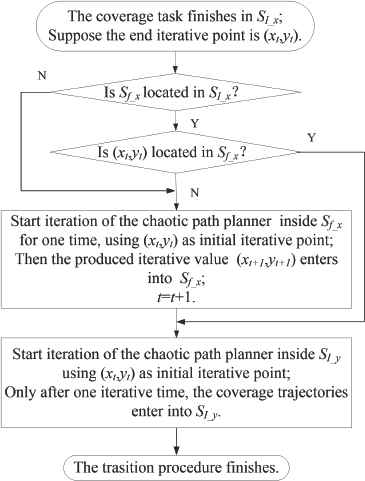
Flowchart of the transition procedure
4.4. Formation of the coverage connected-path
The robot has to cover each SI_x according to a connected-order. The order can be set in a constant sequence to guarantee the complete coverage and avoid overlapping coverage, or in a random sequence to acquire more unpredictable trajectories. A constant sequence should satisfy the following conditions:
- •
The path must include every SI_x to guarantee the complete coverage.
- •
The number of SI_x in the path should be as little as possible to avoid overlapping of coverage.
Though the question can be formulated as a TSP task, it has some difference. For the CCPP problem, each node (sub-region) in the route can be visited for several times to finish the coverage task instead one if only each sub-region owns relatively the same coverage evenness.
4.5. Covering procedure
According to the above designed algorithm, CCPP task in workplace can be achieved as follows.
- (i)
Initialization of CCPP task.
- (a)
Compute the affine parameters [a b c d] of all SI_x and Sf_x, and construct the chaotic path planner of them based on Eq. (3);
- (b)
Set up the total loop time NLoop. Each SI_x being covered for one time is a loop;
- (c)
Set up the total iterative time N1 in one NLoop according to the task requirements;
- (d)
Compute iterative time nI_x of SI_x related to N1 based on their size proportion to the total free area, respectively;
- (e)
Select the covering direction P. P=1: clockwise, P=0: counterclockwise;
- (f)
Select an original point (x0,y0) randomly, and determine the SI_x in which the point is located;
- (g)
Set a parameter NT to record the transition time between two adjacent SI_x during CCPP task, the initial value NT =0.
- (a)
- (ii)
Start the chaotic path planner based on (x0, y0) and produce the covering trajectories in SI_x until the sub-task of CCPP realizes inside.
- (iii)
Select the next SI_x according to the designed coverage connected-path.
- (iv)
Realize the transition procedure based on the designed method mentioned in Section 4.3.
- (v)
Repeat the above procedure (ii)~(iv) until the covering trajectories return to the start SI_x and one loop ends.
- (vii)
Repeat the above procedure (ii)~(v) until all loops end, and the whole CCPP task achieves.
5. Verification of the Proposed Algorithm
Here we assume a case to verify the proposed integrated method for achieving CCPP task. For the sake of simplicity, we select the most common used obstacles to illustrate the feasibility of the algorithm.
Case: as shown in Fig. 8.(a), the size of workplace is 10×10. There is a dark gray obstacle which size is 4×4 seated at the center of workplace. Its coordination of left-bottom corner is (3,3). The requirement is to compute the complete coverage trajectories for CCPP task while avoiding the obstacle, and meet the demands for the special missions.
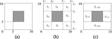
Workplace and the decomposition result (a) original workplace, (b) decomposition into grids Sx, and (c) construction of the iterative sub-regions SI_x
The research resolves the problem based on the strategy discussed in Section 4 step by step.
Fig. 8.(b) shows the decomposition result. The lines L1~L4 are a group of horizontal parallel segmentation lines, while L5~L8 are the vertical ones, among which L1, L4, L5 and L8 are the boundary lines of workplace. After segmentation, the feasible area is divided into eight small adjacent grids Sx, along the boundaries of obstacles and workplace, labeled as SA, SB, SC, SD, SE, SF, SG and SH, respectively.
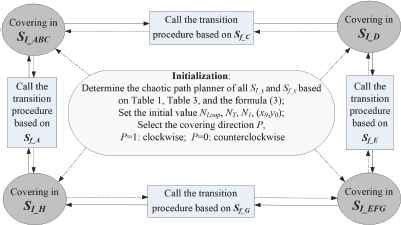
Select the top-bottom direction as merging direction, four iterative sub-regions, namely SI_ABC, SI_H, SI_D, and SI_EFG are constructed respectively, which is shown in Fig. 8.(c), where SI_ABC is formed by SA, SB, and SC, and SI_EFG is formed by SE, SF and SG.
The affine parameters [a b c d] of the four SI_x solved by Eq. (2) for the chaotic path planner are illustrated in Table 1. They are used to construct the chaotic path planner based on Eq. (3) to produce the coverage trajectories inside each SI_x, and part traversing trajectories for transition between two adjacent SI_x.
| SI_x | Affine transformation parameters | |||
|---|---|---|---|---|
| a | b | c | d | |
| SI_ABC | 0 | 7 | 10/2π | 3/2π |
| SI_H | 0 | 3 | 3/2π | 4/2π |
| SI_D | 7 | 3 | 3/2π | 4/2π |
| SI_EFG | 0 | 0 | 10/2π | 3/2π |
Affine transformation parameters SI_x
The safety zone Sf_x between two adjacent SI_x is determined based on their connection relationship and Definition 1. All Sf_x solved according to Fig. 8(b) and Fig. 8(c) are illustrated in Table 2. The affine parameters [a b c d] of the four Sf_x that are solved based on Eq. (2) are listed in Table. 3.
| Adjacent SI_x | Sf_x |
|---|---|
| SI_ABC and SI_D | Sf_C |
| SI_D and SI_EFG | Sf_E |
| SI_EFG and SI_H | Sf_G |
| SI_H and SI_ABC | Sf_A |
Sf_x between two adjacent SI_x
| Sf_x | Affine transformation parameters |
|||
|---|---|---|---|---|
| a | b | c | d | |
| Sf_C | 7 | 7 | 3/2π | 3/2π |
| Sf_E | 7 | 0 | 3/2π | 3/2π |
| Sf_G | 0 | 0 | 3/2π | 3/2π |
| Sf_A | 0 | 7 | 3/2π | 3/2π |
Affine transformation parameters of Sf_x
They will be used to construct the chaotic path planner based on Eq. (3) to produce the transition trajectories between two adjacent SI_x.
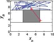
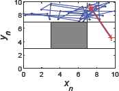
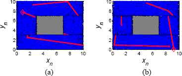
One of the transition procedures, from SI_ABC to SI_D, is illustrated, where Sf_C is their safety zone. The simulation result is shown in Fig. 9. The iterative time n=30, and the original point (x0,y0)=(3,8), which is marked as purple “o” in the figure. The chaotic path planner produces the coverage trajectories in SI_ABC based on (x0, y0), which is shown in Fig. 9.(a). After achieving the coverage task, the final iterative point (xt, yt) marked as red “*”, ending at (4.9972,7.3845), isn’t located in Sf_C. So Sf_C has to be used as the transition region to avoid possible collision of the obstacle. In Fig. 9.(b), start the iterative procedure of the chaotic path planner in Sf_C for one time based on (xt,yt), the next iterative point (xt+1,yt+1) is immediately attracted to Sf_C, which is marked as a red “◇”. Then based on (xt+1, yt+1), start the iterative procedure in SI_D, and after only one time the coverage trajectory enters into it and the transition procedure ceases, which is shown in Fig. 9.(c). The red lines in the figure show the transition trajectories.
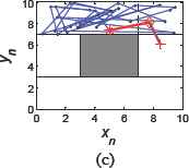
Transition procedure from SI_ABC to SI_D
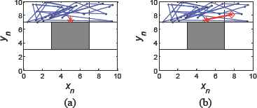
Fig. 9 shows that the transition procedure achieves conveniently and safely. Only after two steps at most, the robot can travel from one SI_x to its adjacent one. The linkage points that collecting the coverage trajectories are produced randomly by the chaotic path planner instead of designing deliberately. The coverage trajectories can avoid obstacle easily because of the installment of the safety zone Sf_x, here is Sf_C. Without it, the robot will collide with the obstacle possibly, which is shown as the red lines in Fig. 10. Of course, when (xt,yt) ends in Sf_C, we can start the iteration of SI_D directly, and transition procedure achieves by only one step without colliding with the obstacle. Fig. 11 shows the case, where (x0,y0)=(8,9). Safety zone is unused under this circumstance.
Circumstance of obstacle collision without using Sf_C
Circumstance of (xt, yt) ending in Sf_C
A coverage connected-path is formed to guide the coverage direction for robot. Fig. 12 shows a constant linkage one. It links the four SI_x in a circle, where the solid arrows indicate clockwise direction, while the dotted arrows indicate counterclockwise direction.
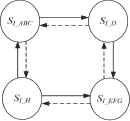
The coverage connected-path
Based on the constructed chaotic path planner and the coverage connected-path, the covering procedure algorithm is designed, which is shown in Fig. 13.
The covering procedure
The algorithm has been simulated with different original point ( x0,y0), iterative time N1, and loop time NLoop. Select the coverage direction P=1. The original value NT=0. According to the designed transition procedure, the possible value of NT after achievement of CCPP task in one loop will assume 4, 5, or 6. Different covering results can be obtained by changing the iterative times of N1 and NLoop.
Fig. 14 and Fig. 15 shows the coverage results in one loop, namely NLoop=1. The marks and lines have the same meaning as the above figures. The results show that from any original point (x0,y0), the robot can achieve the CCPP task conveniently, quickly, and safely by a limited transition time, based on the trajectories produced by the chaotic path planner. The larger the iterative time is, the better the coverage effect can get. Compared with Fig. 14, where N1=420, results in Fig. 15 show a better evenness and completeness at N1=8400. In one loop, whether the N1 is, the NT remains nearly a constant value.
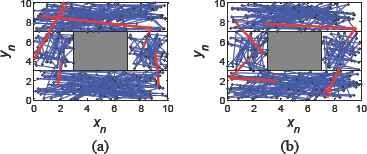
The coverage trajectories at N1=420, NLoop=1 (a) (x0,y0)=(3,8), NT=5 and (b) (x0,y0)=(8,2), NT=6.
The coverage trajectories at N1=8400, NLoop=1 (a) (x0,y0)=(3,8), NT=6 and (b) (x0,y0)=(8,2), NT=6.
Though the original point (x0, y0) can be set randomly, the covering results remain the similar coverage characteristics at the same iterative times, especially when the iterative time assumes a larger value. Because there are little transition times during coverage procedure, the influence of them can be ignored. So the coverage trajectories show almost the same characteristics as the chaotic Standard map, and can satisfy the needs of special missions.
We can further improve the random characteristics of coverage trajectories by increasing the transition frequency among SI_x. Fig. 16 has the same total coverage times as Fig. 15, but in 100 loop times. The transition trajectories, namely the red lines, increase obviously. The circumstance may spoil some distribution characteristics of the coverage trajectories produced by the chaotic path planner. This phenomenon can be coordinated according to the task requirements.
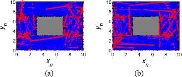
The coverage trajectories at N1=84, NLoop=100 (a) (x0,y0)=(3,8), NT=529 and (b) (x0,y0)=(8,2), NT=536.
Besides the complex computation and low planning efficiency, the common used mirror mapping method is unavailable to the chaotic path planner constructed by the Standard map because of the long distances between two adjacent iterative points produced by the planner29, which can cause the frequently collision with the obstacles. Under this circumstance, the trails produced by the mirror mapping will occupy most part of the coverage trajectories which can totally destroy the chaotic characteristics of them.
6. Conclusion
Taking advantage of the chaotic characteristics of the Standard map, an integrated algorithm has been proposed based on cellular decomposition approach in the obstacles-included environment. The cellular decomposition simplifies the CCPP task into some sub-regions coverage task, using trajectories produced by the chaotic path planner based on the Standard map. The attractor characteristics of the Standard map can deduce the designing complex of obstacles avoidance strategy. The planned coverage trajectories demonstrate almost the same characteristics as the Standard map, such as the completeness, evenness, and randomness or unpredictability, to satisfy the needs of special missions. The designed method owns the following advantages:
- •
No designated linkage points are needed in transition procedure between two adjacent SI_x. They are produced by the chaotic path planner randomly in real time.
- •
Only after two steps at most, the robot can achieve the transition procedure between two adjacent SI_x, so the transition trajectories have little influence to the chaotic characteristics of coverage trajectories.
- •
The obstacles’ avoidance method is very simple. Due to the attractor characteristics of the Standard map, the robot can work in a SI_x forever without going out or colliding with the boundaries of workplace. So no edges’ detection of obstacles and the boundaries of workplace are needed when the robot runs inside a SI_x. Only during transition procedure, the problem of obstacle avoidance is considered.
- •
Establishment of the safety zone between two adjacent SI_x makes transition procedure safe and simple based on the attractor characteristics of the Standard map.
There are also many work to be further researched in the future:
- •
The size of non-rectangular obstacles should be considered. So we have to study the mapping strategy of the Standard map to any size area.
- •
For a target workplace including complex obstacles, the decomposition and transition strategy for the sub-regions have to be explored in depth.
Acknowledgments
This work is supported by the National Natural Science Foundation (NNSF) of China (61473179, 61602280, 61573213); The Natural Science Foundation of Shandong province (ZR2014FM007, ZR2014FQ028, ZR2015CM016 and 2016GGX101027).
References
Cite this article
TY  - JOUR
AU  - Caihong Li
AU  - Zhiqiang Wang
AU  - Chun Fang
AU  - Zhenying Liang
AU  - Yong Song
AU  - Yibin Li
PY  - 2018
DA  - 2018/08/13
TI  - An Integrated Algorithm of CCPP Task for Autonomous Mobile Robot under Special Missions
JO  - International Journal of Computational Intelligence Systems
SP  - 1357
EP  - 1368
VL  - 11
IS  - 1
SN  - 1875-6883
UR  - https://doi.org/10.2991/ijcis.11.1.100
DO  - 10.2991/ijcis.11.1.100
ID  - Li2018
ER  -