
An improved chaotic firefly algorithm for global numerical optimization
- DOI
- 10.2991/ijcis.2018.25905187How to use a DOI?
- Keywords
- Firefly algorithm; chaos; global optimization; nature-inspired algorithms; exploitation; exploration
- Abstract
Firefly algorithm (FA) is a prominent metaheuristc technique. It has been widely studied and hence there are a lot of modified FA variants proposed to solve hard optimization problems from various areas. In this paper an improved chaotic firefly algorithm (ICFA) is proposed for solving global optimization problems. The ICFA uses firefly algorithm with chaos (CFA) as the parent algorithm since it replaces the attractiveness coefficient by the outputs of the chaotic map. The enhancement of the proposed approach involves introducing a novel search strategy which is able to obtain a good ratio between exploration and exploitation abilities of the algorithm. The impact of the introduced search operator on the performance of the ICFA is evaluated. Experiments are conducted on nineteen well-known benchmark functions. Results reveal that the ICFA is able to significantly improve the performance of the standard FA, CFA and four other recently proposed FA variants.
- Copyright
- © 2018, the Authors. Published by Atlantis Press.
- Open Access
- This is an open access article under the CC BY-NC license (http://creativecommons.org/licences/by-nc/4.0/).
1. Introduction
Many real-world optimization problems are formulated as global optimization problems. These problems are difficult for solving because they are usually highly nonlinear with multiple local optimums. As the number of dimensions increases the search space of a problem grows exponentially and its properties may change 1. Therefore, exploring the entire search space efficiently is a complex task. Most deterministic optimization techniques are heavily interrelated to structure of the solution space and hence it is hard to generalize them for all types of optimization problems. Also, these methods can be simply trapped in the local optimum since they are local search algorithms.
On the other hand, metaheuristic algorithms have been shown as efficient tools to solve computationally hard problems. These algorithms are problem independent optimization methods which use some randomness in their strategies in order to more easily avoid local optimums 2. The superiority of majority of metaheuristc algorithms comes from the fact that they imitate the best processes in nature. Over the last three decades more than a dozen of notable metaheuristic algorithms have been proposed 3,4. Prominent members are genetic algorithm (GA) and differential evolution (DE) method which use mechanisms inspired by biological evolution, such as reproduction, mutation, recombination, and selection. There are also many efficient algorithms inspired by nature which are based on mimicking the so-called swarm intelligence characteristics of biological agents such as birds, fish or ants. Well studied examples are particle swarm optimization (PSO) 5, artificial bee colony (ABC) 6, firefly algorithm (FA) 7, cuckoo search (CS) 8, etc. After their invention, metaheuristics have been modified or hybridized with other methods in order to make their performances more successful 9, 10, 11,12. Specially, there are a lot of improved variants of some prominent metaheuristic algorithms proposed for global optimization 13, 14, 15, 16, 17, 18. However, studies show that it is not possible to develop a general purpose algorithm that reaches optimal solution for all types of optimization problems 19. Hence, it is of great importance to find the best and most efficient algorithm for some types of optimization problems.
The firefly algorithm is designed to solve numerical optimization problems in 2008 by Yang 2. It is inspired by communication behavior of flashing fireflies. The FA is effective metaheuristic technique, which has simple concept and easy implementation. Therefore the FA has been studied by many researchers and new FA variants have been described to solve different classes of optimization problems, such as continuous, combinatorial, constrained, multi-objective, dynamic and noisy optimization 20,21,22,23,24.
In spite of the fact that the FA has been shown to be an efficient optimization technique, there is still an insufficiency in the FA regarding its solution search equation. It is observed that the FA search equation can be overly random in the beginning of the search process due to the usage of different values of its randomization term to update each solution variable. Consequently FA search equation is good for exploration, but poor for exploitation in the first generations of the search process, which can considerably deteriorate the optimization results.
An improved chaotic firefly algorithm (ICFA) for global numerical optimization is presented to overcome the above drawback. Three modifications are made to the standard FA with the intention to modify its behaviour in a bound-constrained search space. Firstly, to improve the exploitation ability of the FA, a new movement equation is employed in the initial generations of a search. Secondly, considering the previous work on the FA, the ICFA uses the chaotic map in order to tune the attractiveness parameter and consequently produce useful diversity in the population. The third modification is related to the usage of the improved method to handle the boundary constraints. The ICFA is tested to solve 19 well-known benchmark functions. Numerical results reveal that the ICFA is superior to the standard FA and five other FA variants.
The paper is organized as follows. Section 2 presents the standard FA. A brief literature review of FA and its variants for numerical optimization is presented in Section 3. The details of our proposed ICFA are described in Section 4. Section 5 presents benchmark problems, parameter settings and analysis of the obtained results. In Section 6 the conclusion is drawn.
2. Firefly algorithm
In the population of fireflies, each member represents a candidate solution in the search space 20. Fireflies move towards the more attractive individuals and find potential candidate solutions. A firefly’s attractiveness is proportional to its light intensity or brightness, which is usually measured by the fitness value. The framework of FA is given as Algorithm 1, restated from Ref. 2.
Important details related to the movement equation used in the FA for unconstrained functions with higher variables are explained as follows. If solution xj has better objective function value than xi, the parameter values xik are updated by the following rule described in Ref. 2:
Create an initial population of solutions xi, i = 1,2,…,SP while (t < Maximum Cycle Number (MCN)) do Move fireflies: For each solution xi, i = 1,2,…,SP, compare it with other all solutions xj, j = 1,2,…,SP of the population. If the objective function value of xj is less than xi, then move xi towards xj in all D dimensions, apply control of the boundary conditions on the created solution and evaluate it. Rank the fireflies: Sort the population of solutions according to their objective function values. t = t + 1. end while |
Framework of the FA
The second term on the right-hand of Eq. (1) is due to the attraction. In this term rij = ||xi − xj||2 is the l2 norm or Cartesian distance, while control parameter β0 is attractiveness coefficient, parameter βmin is minimum value of β and parameter γ is absorption coefficient. The parameter β0 represents attractiveness at r = 0, while the parameter γ characterizes the variation of the attractiveness. The suggested values for parameter β0 is 1 and for parameter βmin is 0.2 2. For most applications γ = O(1) can be employed 25.
The third term of Eq. (1) is randomization term. In this term α ∈ [0,1] is randomization parameter and randk is a random number uniformly distributed between 0 and 1. Also, in this term sk = |uk − lk| is the length scale for the kth variable of the solution, where lk and uk are the lower and upper bound of the parameter xik. In Ref. 2 it was noted that parameter α should be linked with scales and that the steps should not be too large or too small.
The parameter α controls the step sizes of the random walks 26. Although in Ref. 25 it was noticed that for most problems a fixed value of randomization parameter from range (0, 1) can be used, later findings pointed out that α needs to be reduced gradually during iterations. A good way to calculate α is given by
The update process is finished when the boundary constraint-handling mechanism is applied to the created new solution. The boundary constraint-handling mechanism used in the FA is described by
Exploitation and exploration are important components of the FA, as well as of any metaheuristic algorithm 27. The process of focusing the search on a local region by using the information of previously visited good solutions is exploitation. On the other hand, exploration is the process of creating solutions with plenty of diversity and far from the actual solutions. Exploitation and exploration are fundamentally conflicting processes. In order to be successful, a search algorithm needs to establish a good ratio between these two processes. The randomization term of the FA search equation gives an ability to the algorithm to get out of a local optimum in order to seek on a global scale 26. In terms of the attraction mechanism, fireflies can automatically subdivide themselves into several subgroups, and each group can search around a local region. These advantages indicate that the FA is good at exploration as well as exploitation.
3. Brief review of FA
Yang tested the performance of FA for optimizing multimodal numerical optimization problems 7. The performance of the FA, when it was applied to ten standard benchmark functions, has been compared with the performance of the PSO and DE. The experimental results revealed that FA outperformed both algorithms. But, when being applied to multimodal continuous optimization problems, original FA gets trapped in the local optimum due to unsatisfactory settings of its control parameters, which remain fixed throughout all iterations. In Ref. 7 it was concluded that it is possible to improve the solution quality and convergence speed by reducing the randomness gradually. Some of the recent FA variants developed to solve numerical optimization problems more efficiently are presented as follows.
Gandomi et al. at 2013 developed FA variants which use chaotic maps 28. In Ref. 28, twelve different chaotic maps are used to improve the attraction term of the algorithm. The experimental results pointed out that tuning of the attractiveness coefficient is more effective than tuning light absorption coefficient. It was concluded that the most suitable choice to tune the attractiveness coefficient is the Gauss map. Therefore, at the end of each CFA iteration, the value of parameter β0 is updated by
In the same year, Fister et al. proposes to use quaternion for the representation of individuals into FA (also QFA) in order to avoid any stagnation 29. The proposed QFA has been applied to optimize a test-suite consisting of ten standard functions with 10, 30 and 50 variables. The results have shown that QFA performs better than the standard FA and comparable with other state of the art algorithms, such as DE, ABC and BA.
A wise step strategy FA (WSSFA) is proposed in 2014 30. In the WSSFA, each firefly in the swarm has an independent step parameter, which considers the information of firefly’s previous best and the global best positions. A variable step FA (VSSFA) which employs a dynamic strategy to adjust randomization parameter was proposed in 2015 in Ref. 31. Experiments on standard benchmark functions showed that the VSSFA and WSSFA reached better solutions than the standard FA on some test functions 30,31.
Wang et al. in 2016 developed a novel FA variant (RaFA) which uses a random attraction model and a Cauchy mutation operator 32. Simulation results on standard benchmark functions have proven that RaFA performs better than the standard FA and two other improved FAs. Zhang et al. in the same year designed the hybrid firefly algorithm (HFA) which combines the advantages of both the firefly algorithm (FA) and the differential evolution (DE) 33. A diverse set of 13 high-dimensional benchmark functions with 30 variables were used to test the performance of the HFA. The experimental results revealed that HFA outperformed the original FA, DE and PSO algorithms in the terms of accuracy of solutions, with faster convergence speed.
A new FA variant, called FA with neighbourhood attraction (NaFA), was developed by Wang et al. in 2017 17. In this approach, each firefly was attracted by other brighter fireflies selected from a limited neighbourhood. Experiments on 13 standard benchmark functions with 30 variables showed that the NaFA obtained better solutions than the standard FA and seven other FA variants.
4. The proposed approach: ICFA
Performance of the FA basically depends on its search equation which is a mutation operator used for both local and global search 26. However, achieving optimal balance between local and global search may depend on a lot of factors, such as the setting of algorithm-dependent parameters and the problem to be solved. Furthermore, different amounts of exploration and exploitation are needed during the search process, considering the fact that different values of control parameters might be optimal at different stages of the search 27. In order to accomplish more efficient search process the proposed ICFA introduces a novel movement strategy. The remaining modification is related to boundary constraints. The details of each modification and implementation steps of the ICFA are presented as follows.
4.1. Modifications of the movement
Diversity of a population is a key factor for achieving a proper balance between exploitation and exploration. The population of solutions which are different from each other is a precondition for exploration, while small diversity provides the final results as near as much to the global optimum. The strength of perturbations in the FA is controlled by the randomization parameter. The values of the randomization term of Eq. (1) are higher in the initial stages of the search process and they are gradually reduced during the search. Hence the diversity of a population is greater in the first generations of the search process. Consequently exploration ability of Eq. (1) is greater in these generations than in the later ones. It is observed that for some problems the usage of different values of the randomization term for each solution variable produces too much randomness in the first generations of the search process. Therefore in these cases a less attractive diverse population is obtained. To sum up, the solution search equation described by Eq. (1) can be overly random, and therefore good at exploration, but lack at exploitation in the initial generations of the search.
To overcome this drawback, the ICFA modifies the FA search equation presented by Eq.(1). The novel mutation operator is given by
The second term in the right-hand side of Eq. (6) is equal to the attraction term of Eq. (1) multiplied by a factor of 0.5. In addition, considering the previous work related to the CFA variants, in the attraction term of Eq. (6) chaotic sequences are employed in order to tune the attractiveness coefficient β0. Hence at the end of each iteration t the outputs of the Gauss chaotic map βchaos(t) generated by Eq. (5) are used.
The third term in the right-hand side of Eq. (6) is equal to the difference vector formed by the other two solutions multiplied by a factor of 0.5. In this term rand1 and rand2 are integers randomly generated within the range [1, SP], which are also different from index i. Similar as in DE algorithm, adding the vector subtraction might lead to better perturbation of solutions than one-difference vector-based strategies 34.
The fourth term in the right-hand side of Eq. (6) is randomization term. In this term r is a random number in (0, 1). It can be noticed that the same random number is used for all dimensions. Comparing the randomization terms of Eq. (1) and Eq. (6), Eq. (1) can have a larger search space due to independent updating of each dimension. On the other hand, Eq. (6) has a smaller search space due to the same random number being employed for all dimensions. Also, in this term the value α(t) is calculated by Eq. (3) at the end of each iteration.
While different implementation of the randomization terms of Eq. (1) and Eq. (6) may seem of minor importance, the implications on the FA performance are quite beneficial. In fact, differences among individuals of the population are reduced by using Eq. (6) as a consequence of reducing the space where the newly created solution can be. Therefore this modification prevents the algorithm to provide too much exploration in the initial iterations of the search process. However, the randomization parameter is gradually reduced during the search, and at one point using the same random number in the randomization term of Eq. (6) can provide too much exploitation and consequently premature convergence. Therefore in order to adjust the exploitation and exploration during the search process, the ICFA uses both mutation operators which are described by Eq.(6) and Eq.(1). In the initial generations of the search Eq. (6) is used, while Eq. (1) is employed in the remaining generations. The ICFA introduces a new control parameter in order to determine the number of iterations in which it is fruitful to use the mutation operator described by Eq. (6). This parameter is called percent o f generations (pg) and it takes value between 0 and 1. Therefore, the ICFA uses Eq. (6) in the first pg · MCN iterations of a search process, while in the remaining iterations it employs Eq. (1). It is worth noting that the vector subtraction is not included in Eq. (1) since the convergence may be slowed down by additional randomness provided by it.
Observe that the parameter pg has a significant role in balancing the exploration and exploitation of the candidate solution search. When pg takes 0, the search is based only on Eq. (1), i. e. the ICFA is equal to the CFA. When pg increases from zero to a certain value, the exploitation ability of the ICFA will also increase appropriately. The reason lies in the fact that Eq. (6) has a smaller search space in comparison to Eq. (1) due to the same random number used for all dimensions in the randomization term. However, pg should not be too large since it might result in relatively weakening the exploration ability of the ICFA.
4.2. Boundary constraint-handling method
Using the efficient boundary constraint-handling mechanism can greatly contribute to successful optimization performance of a search algorithm. According to Eq. (4), the standard FA can be easily caught in the local minimum if there are a lot of solutions focused in the extreme values of the search space. In order to overcome this, an improved boundary constraint-handling mechanism which creates a diverse set of values can be employed.
There are several improved boundary constraint-handling methods which were successfully used in order to help maintaining diversity in the population 35. In the ICFA the method for handling the boundary constraints is given by 36:
Initial control parameters of the ICFA, including: SP, MCN, α0, βmin, β0, γ, θ, pg. Initialize SP population solutions xi (i = 1,2,…,SP) randomly in the search space. Evaluate each solution in the initial population using the objective function. t=0 while t < MCN do for i = 1 to SP do for j = 1 to SP do if (f(xj) < f(xi)) then if (t < pg · MCN) then Move xi toward xj according to Eq. (6) else Move xi toward xj according to Eq. (1) end if Apply control of the boundary conditions on the created solution xi by Eq. (8) and evaluate it end if end for end for for k = 1 to D do Update the αk,t value by Eq. (3) end for Update the βt value by Eq. (7) Rank the solutions and find the current best t = t + 1 end while |
Pseudo-code of the ICFA
4.3. The pseudo-code of the ICFA
The proposed ICFA uses six specific control parameters to manage the search process: the initial randomization α0, the initial maximum attractiveness β0, the parameter βmin, the absorption coefficient γ, the cooling factor θ and the parameter pg which determines the number of initial iterations in which the novel mutation operator described by Eq. (6) is used to update a solution. The ICFA also employs the size of population SP and maximum cycle number MCN, which are common control parameters for all nature inspired algorithms. The computational time complexity of the ICFA is equal to those of the standard FA, i.e. it is O(MCN · SP2 · f), where O(f) is the computational time complexity of the fitness evaluation function. The pseudo code of the proposed ICFA is presented in Algorithm 2.
5. Experimental study
This section presents the detailed evaluation of the proposed ICFA. In order to demonstrate the performance of the ICFA, 19 well-known benchmark functions are used 37. The Table 1 presents the name of the benchmark function (column 1), its formula (column 2) and search space range (column 3). Listed high-dimensional benchmark functions can be divided into two categories according to their features: unimodal functions (f1 − f7) and multimodal (f8 − f19) functions. A function is unimodal if it has a single optimal solution. Multimodal functions are more difficult test problems, since they have more than one local optimum. However, although functions f1 − f7 represent unimodal functions in 2D or 3D search space, they can be seen as multimodal functions in high-dimensional cases 38.
| Function | Formula | Search range |
|---|---|---|
| Sphera |
|
[−100,100]D |
| Schwefel 2.22 |
|
[−10,10]D |
| Schwefel 1.2 |
|
[−100,100]D |
| Schwefel 2.21 | f4(x) = max|xi|, 1 ≤ i ≤ D | [−100,100]D |
| Rosenbrock |
|
[−30,30]D |
| Step |
|
[−100,100]D |
| Quartic |
|
[−1.28,1.28]D |
| Schwefel 2.26 |
|
[−500,500]D |
| Rastrigin |
|
[−5.12,5.12]D |
| Ackeley |
|
[−32,32]D |
| Griewank |
|
[−512,512]D |
| Penalized 1 |
|
[−50,50]D |
| Penalized 2 |
|
[−50,50]D |
| Alpine |
|
[−10,10]D |
| Periodic |
|
[−10,10]D |
| Xin-She Yang |
|
[−2π,2πD |
| Himmelblau |
|
[−5,5]D |
| Styblinski-Tank |
|
[−5,5]D |
| W / Wavy |
|
[−π,π]D |
Benchmark functions used in the experiments, where D is the problem dimension.
There are three experiments for assessing the performance of ICFA. First experiment is used to investigate the impact of the introduced search strategy described by Eq. (6) on the ICFA performance. Therefore different values of the parameter pg were tested in order to determine an appropriate choice of this parameter. Second experiment is employed to evaluate the performance of the ICFA when it is compared to FA variants. Two types of comparisons were considered. The first type is a direct comparison between the ICFA and our implementation of the standard FA and CFA. The second type of comparison is an indirect comparison, where the results of other FA approaches were taken from the specialized literature and compared with those reached by the ICFA. The third experiment is used to consider the exploration and exploitation abilities of the proposed algorithm.
5.1. Investigation of the parameter pg
The parameter pg is a new control parameter introduced to maintain the diversity of the population and therefore control exploration/exploitation balance of the algorithm. It determines the number of initial iterations in which the new movement equation described by Eq. (6) is used to update a solution, and it takes value between 0 and 1. If pg takes 0, the ICFA is equal to the CFA which uses the improved boundary handling method, i. e. the search is based only on Eq. (1). When pg increases from zero to a certain value, the number of initial iterations in which the search is based on Eq. (6) will increase, as well. If pg takes 1, the search is based only on Eq. (6). Therefore the parameter pg is an important factor in the performance of the ICFA. In this subsection different values of pg were tested in order to explore the effects of pg on the performance of the ICFA. An appropriate choice of pg could be determined from the performed tests.
The parameter SP was set to 20 and the MCN was set to 2000. The specific parameter values are the following: α0 = 0.8, β0 is a random number from (0, 1), βmin = 0.2, γ = 1 and θ = (10−11/0.9)2/MCN. Then, pg was set to 0, 0.1, 0.2, and 0.3. For each value of pg, the ICFA was run 30 times for each benchmark function with D = 30. The mean best values and standard deviation values were recorded and these values are shown in Table 2.
| F. | pg = 0 | pg = 0.1 | pg = 0.2 | pg = 0.3 |
|---|---|---|---|---|
| Mean(std.) | Mean(std.) | Mean(std.) | Mean(std.) | |
| f1 | 1.20E-39(3.07E-40) | 1.24E-39(2.36E-40) | 1.15E-03(4.25E-03) | 2.09E-02(2.41E-02) |
| f2 | 1.55E-20(1.72E-21) | 1.54E-20(1.60E-21) | 4.48E-02(6.08E-02) | 8.32E-02(5.14E-02) |
| f3 | 1.65E-77(5.92E-78) | 1.45E-77(3.67E-78) | 4.29E-03(2.08E-02) | 2.95E-02(6.07E-02) |
| f4 | 1.61E-20(2.72E-21) | 1.67E-20(2.47E-21) | 2.90E-03(8.52E-03) | 3.34E-02(3.27E-02) |
| f5 | 3.17E+01(1.80E+01) | 2.53E-05 (3.55E-05) | 8.81E-06(1.30E-05) | 3.25E-01 (3.93E-01) |
| f6 | 4.33E-01(4.95E-01) | 0.0E+00(0.0E+00) | 0.0E+00(0.0E+00) | 0.0E+00(0.0E+00) |
| f7 | 5.81E-02 (1.42E-02) | 1.90E-04(9.66E-05) | 1.22E-04(1.52E-04) | 1.39E-04 (1.88E-04) |
| f8 | 4.74E+03(5.48E+02) | 3.82E-04(1.25E-12) | 3.82E-04(1.14E-12) | 3.87E-04(2.28E-05) |
| f9 | 5.76E+01(2.20E+01) | 5.92E-17(3.19E-16) | 1.68E-04(8.61E-04) | 1.94E-02(3.13E-02) |
| f10 | 2.17E-14 (6.92E-15) | 2.60E-14(1.07E-14) | 1.81E-03(5.37E-03) | 3.59E-02(3.54E-02) |
| f11 | 3.53E-03(5.53E-03) | 3.70E-18(1.99E-17) | 8.34E-03(2.99E-02) | 5.59E-02(7.95E-02) |
| f12 | 6.91E-03(2.59E-02) | 1.57E-32(5.47E-48) | 8.66E-06(1.92E-05) | 2.40E-04(3.40E-04) |
| f13 | 4.26E-03(1.17E-02) | 1.42E-31(4.33E-33) | 1.97E-04(4.57E-04) | 2.90E-03(4.77E-03) |
| f14 | 4.62E-02(8.08E-02) | 2.02E-18(2.61E-18) | 2.05E-04(4.72E-04) | 3.83E-03(2.72E-03) |
| f15 | 1.22E-41(2.55E-42) | 1.22E-41(1.98E-42) | 1.018E-05(3.98E-05) | 5.20E-04(8.37E-04) |
| f16 | 6.72E-12(1.33E-12) | 3.51E-12(6.79E-27) | 3.51E-12(1.45E-26) | 3.51E-12(2.46E-16) |
| f17 | −68.72 (2.94E+00) | −78.33(2.85E-14) | −78.33(4.04E-14) | −78.30(3.78E-02) |
| f18 | −1069.90(3.40E+01) | −1174.99(2.59E-13) | −1174.99(3.35E-13) | −1174.98(1.37E-04) |
| f19 | 4.25E-01(6.49E-02) | 0.0E+00(0.0E+00) | 8.48E-06 (4.55E-05) | 7.47E-05(1.09E-04) |
Mean best objective function values and standard deviation values achieved by the ICFA with different pg values with D = 30. The best results are indicated in bold.
From the results presented in Table 2 it can be seen that the performance of the ICFA depends on the value of the parameter pg. For a majority of test problems the ICFA obtains better or similar results when pg = 0.1. The only exception are for problems f5 and f7 where ICFA with pg = 0.2 yields the best mean and standard deviation values. The performance of the ICFA was deteriorated almost for all test problems when the pg is set to 0.3. Hence the ICFA results when the value of pg is higher than 0.3 are not presented in this study. The Friedman test was performed in order to find the suitable pg value. In order to perform the Friedman test, we rank the ICFA with different pg values according to the mean values in Table 2. The best rank is indicated in bold. It can be noticed that pg = 0.1 reaches the best rank.
| ICFA | Mean rank |
|---|---|
| pg = 0.1 | 1.58 |
| pg = 0.2 | 2.24 |
| pg = 0 | 2.92 |
| pg = 0.3 | 3.26 |
Mean rank achieved by the Friedman test for ICFA with different pg values.
Figure 1 presents convergence graphs associated with the mean results among 30 runs obtained by the ICFA with different pg values for the six selected functions. From Figure 1 it can be seen that for majority problems the ICFA with pg = 0.1 converges faster than that with other pg values. Therefore the parameter pg is set to 0.1 in the further tests.
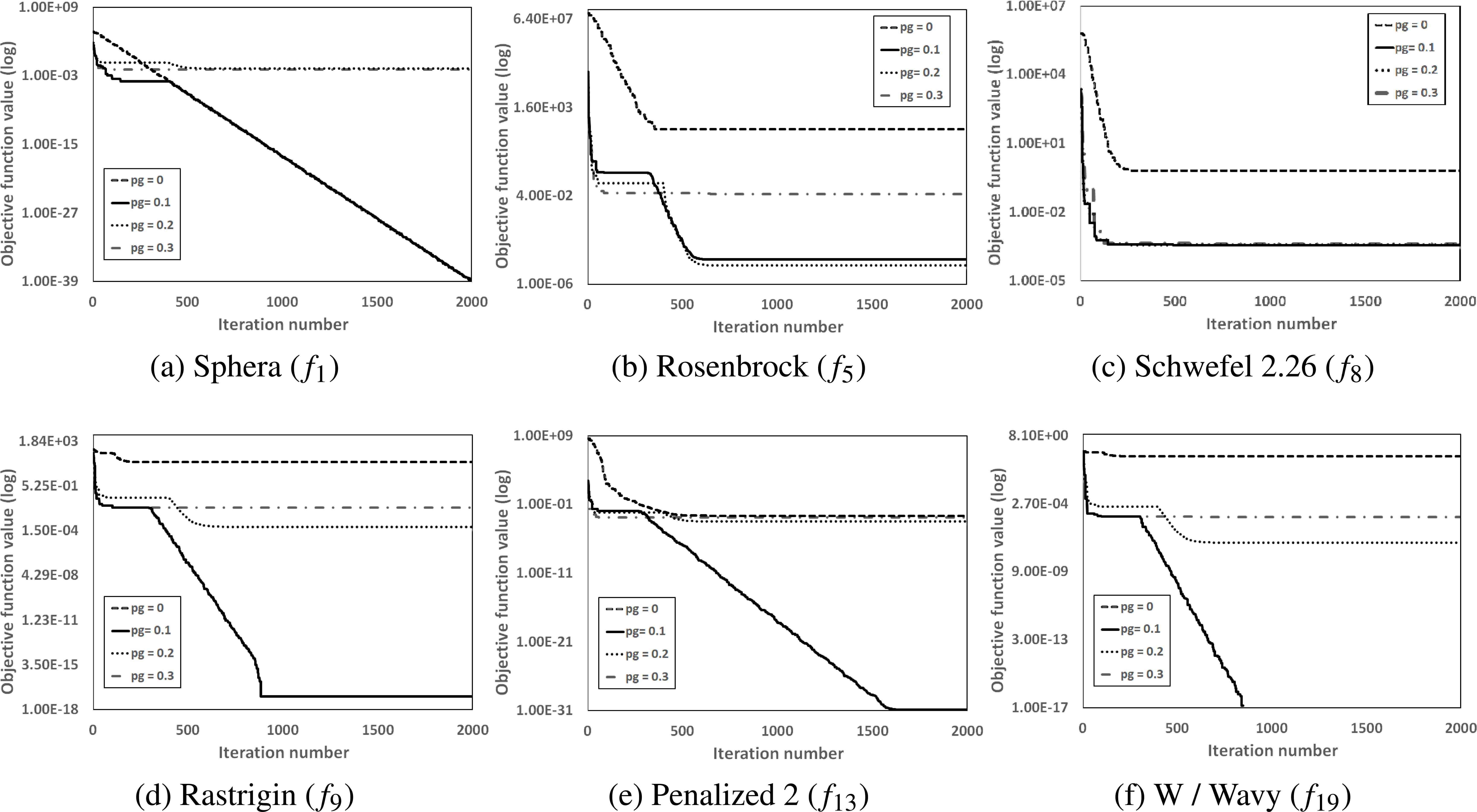
The convergence graphs of the mean results obtained by the ICFA with different pg values on the selected functions with 30 variables.
5.2. Direct comparison with the standard FA and CFA
A direct comparison between the ICFA and standard FA through the 19 benchmark functions with 30 and 50 variables is presented in this subsection. Additionally, since the ICFA uses the CFA as the parent algorithm, the results of the CFA are also included in the comparison with the proposed ICFA. Each algorithm was implemented in Java programming language on a PC with Intel(R) Core(TM) i5-4460 3.2GHz processor with 16GB of RAM and Windows OS. To explore the effectiveness of the usage of the modified FA equation alone, in our implementation of the CFA an improved method for handling boundary constraints described by Eq. (8) is used. In the other words, the difference between the ICFA and CFA is the usage of the modified FA operator described by Eq. (6) in the first ten percent of the maximum number of generations.
For the FA, CFA and ICFA the values of parameter SP was set to 20. For each algorithm, the parameter MCN was set to 2000 for benchmark functions with 30 and 2500 for benchmark functions with 50 variables. In the experiments, the FA uses the same specific parameter settings as those suggested in 2. These values are the following: α0 = 0.2, β0 = 1.0, βmin = 0.2, γ = 1 and θ = (10−4/0.9)1/MCN. The specific parameter values utilized by the CFA and ICFA in all the experiments are the following: α0 = 0.8, β0 is a random number from (0, 1), βmin = 0.2, γ = 1 and θ = (10−11/0.9)2/MCN. For each benchmark function, each algorithm was run independently 30 times. It is important to note that for each tested algorithm (the FA, CFA and ICFA), in each generation the total number of attractions for all fireflies is SP · (SP − 1)/2. Consequently, the maximum number of function evaluations per generation is SP · (SP − 1)/2. Therefore the maximum number of function evaluations (MaxFEs) per run obtained by each tested algorithm, the FA, CFA and ICFA is MaxFEs = 20 · 19 · 0.5 · 2000 = 380000 for benchmark functions with 30 variables and MaxFEs = 20·19·0.5·2500 = 475000 for benchmark functions with 50 variables.
Three metric are used to estimate the performances of the FA, CFA and ICFA. The performance comparison concerning the robustness and convergence speed are conducted between the FA, CFA and ICFA. The mean and corresponding standard deviation values of 30 independent runs are used to determine the quality or accuracy of the solutions obtained by these algorithms. The convergence speed of each algorithm is compared by the metric AVEN 39. This metric records the average number of function evaluations needed to achieve the acceptable value. The convergence speed is faster if the value of AVEN is smaller. The robustness or reliability of each algorithm is compared by measuring the success rate (SR%). This rate denotes the ratio of successful runs in the 30 independent runs. A successful run means the algorithm reaches a solution whose objective function value is less than the corresponding acceptable value. The robustness of the algorithm is better if the value of SR is greater.
Mean and standard deviation results for benchmark functions with 30 and 50 variables are reported in Table 4 and Table 5. Wilcoxon’s rank sum test at a 0.05 significance level was conducted between the compared algorithm and the ICFA. The result of the test is represented as ”+/≈/-”, which means that the corresponding algorithm is significantly better than, statistically similar to, and significantly worse than the ICFA.
| Function | FA |
CFA |
ICFA |
|||
|---|---|---|---|---|---|---|
| Mean | Std. | Mean | Std. | Mean | Std. | |
| f1 | 8.22E-05 | (1.83E-05)- | 1.20E-39 | (3.07E-40)≈ | 1.24E-39 | (2.36E-40) |
| f2 | 4.39E-03 | (4.46E-03)- | 1.55E-20 | (1.72E-21)≈ | 1.54E-20 | (1.60E-21) |
| f3 | 7.26E-08 | (2.50E-08)- | 1.65E-77 | (5.92E-78)≈ | 1.45E-77 | (3.67E-78) |
| f4 | 4.71E-03 | (6.53E-04)- | 1.61E-20 | (2.72E-21)≈ | 1.67E-20 | (2.47E-21) |
| f5 | 5.40E+01 | (6.04E+01)- | 3.17E+01 | (1.80E+01)- | 2.53E-05 | (3.55E-05) |
| f6 | 3.00E-01 | (5.85E-01)- | 4.33E-01 | (4.95E-01)- | 0.00E+00 | (0.00E+00) |
| f7 | 6.26E-01 | (2.78E-01)- | 5.81E-02 | (1.42E-02)- | 1.90E-04 | (9.66E-05) |
| f8 | 4.93E+03 | (6.99E+02)- | 4.74E+03 | (5.48E+02)- | 3.82E-04 | (1.25E-12) |
| f9 | 4.96E+01 | (1.18E+01)- | 5.76E+01 | (2.20E+01)- | 5.92E-17 | (3.19E-16) |
| f10 | 2.14E-03 | (1.59E-04)- | 2.17E-14 | (6.92E-15)≈ | 2.60E-14 | (1.07E-14) |
| f11 | 5.76E-03 | (5.32E-03)- | 3.53E-03 | (5.53E-03)- | 3.70E-18 | (1.99E-17) |
| f12 | 2.28E-07 | (3.76E-08)- | 6.91E-03 | (2.59E-02)- | 1.57E-32 | (5.47E-48) |
| f13 | 6.29E-06 | (1.43E-02)- | 4.26E-03 | (1.17E-02)- | 1.42E-31 | (4.33E-33) |
| f14 | 3.03E+00 | (1.12E+00)- | 4.62E-02 | (8.08E-02)- | 2.02E-18 | (2.61E-18) |
| f15 | 8.25E-07 | (1.08E-07)- | 1.22E-41 | (2.55E-42)≈ | 1.22E-41 | (1.98E-42) |
| f16 | 5.39E-12 | (6.62E-13)- | 6.72E-12 | (1.33E-12)- | 3.51E-12 | (6.79E-27) |
| f17 | −70.3214 | (2.06E+00)- | −68.7194 | (2.94E+00)- | −78.3323 | (2.85E-14) |
| f18 | −1036.4451 | (3.75E+01)- | −1069.9020 | (3.40E+01)- | −1174.9850 | (2.59E-13) |
| f19 | 3.21E-01 | (5.67E-02)- | 4.25E-01 | (6.49E-02)- | 0.00E+00 | (0.00E+00) |
| +/≈/- | 0/0/19 | 0/6/13 | ||||
Mean and standard deviation values obtained by the FA, CFA and ICFA on 19 benchmarks with D = 30.
| Function | FA |
CFA |
ICFA |
|||
|---|---|---|---|---|---|---|
| Mean | Std. | Mean | Std. | Mean | Std. | |
| f1 | 1.61E-04 | (1.32E-05)- | 3.20E-39 | (3.88E-40)≈ | 3.21E-39 | (4.02E-40) |
| f2 | 1.07E-03 | (1.88E-03)- | 3.32E-06 | (1.79E-05)- | 3.34E-20 | (2.79E-21) |
| f3 | 5.29E-07 | (1.52E-07)- | 1.90E-76 | (5.96E-77)≈ | 1.97E-76 | (6.78E-77) |
| f4 | 1.09E-02 | (2.07E-03)- | 1.99E-03 | (4.59E-03)- | 1.28E-04 | (4.96E-04) |
| f5 | 9.31E+01 | (1.00E+02)- | 1.21E+02 | (1.12E+02)- | 9.14E-06 | (1.28E-05) |
| f6 | 5.33E-01 | (8.84E-01)- | 9.33E-01 | (1.81E+00)- | 0.00E+00 | (0.00E+00) |
| f7 | 5.78E-01 | (2.51E-01)- | 1.34E-01 | (3.80E-02)- | 2.18E-04 | (2.04E-04) |
| f8 | 8.91E+03 | (7.18E+02)- | 8.59E+03 | (1.06E+03)- | 6.36E-04 | (4.67E-12) |
| f9 | 9.29E+01 | (2.26E+01)- | 1.04E+02 | (2.52E+02)- | 1.78E-16 | (7.03E-16) |
| f10 | 2.92E-03 | (2.33E-04)- | 3.51E-14 | (8.29E-15)≈ | 3.83E-14 | (9.14E-15) |
| f11 | 3.69E-04 | (3.60E-05)- | 1.23E-03 | (2.76E-03)- | 4.44E-17 | (6.78E-17) |
| f12 | 2.07E-02 | (2.93E-02)- | 8.29E-03 | (2.11E-02)- | 1.06E-32 | (1.69E-33) |
| f13 | 9.89E-02 | (1.40E-02)- | 4.26E-03 | (1.17E-02)- | 1.69E-31 | (1.37E-32) |
| f14 | 2.47E-02 | (1.92E-02)- | 1.53E-02 | (3.13E-02)- | 8.31E-18 | (8.50E-18) |
| f15 | 2.61E-06 | (2.45E-07)- | 3.17E-41 | (4.75E-42)≈ | 3.01E-41 | (3.83E-42) |
| f16 | 1.80E-20 | (1.98E-21)- | 2.59E-20 | (8.49E-21)- | 1.21E-20 | (1.28E-34) |
| f17 | −69.2281 | (2.47E+00)- | −68.0031 | (1.80E+00)- | −78.3323 | (3.83E-14) |
| f18 | −1720.8113 | (4.46E+01)- | −1750.0273 | (4.79E+01)- | −1958.3083 | (3.32E-13) |
| f19 | 3.57E-01 | (5.62E-02)- | 4.32E-01 | (4.89E-02)- | 0.00E+00 | (0.00E+00) |
| +/≈/- | 0/0/19 | 0/4/15 | ||||
Mean and standard deviation values obtained by the FA, CFA and ICFA on 19 benchmarks with D = 50.
The results regarding the benchmark functions with 30 variables indicate that the ICFA is significantly better than the FA and CFA in most cases. Specifically, the ICFA is significantly better than the FA and CFA on 19 and 13 test problems out of 19 benchmarks, respectively. It is similar to the CFA on 6 test problems. From the results of the benchmark functions with 50 variables, it is clear that the ICFA also outperforms the FA and CFA in the majority of cases. Particularly, it can be observed that the ICFA is significantly better than the FA on each test problem. With respect to the CFA, the ICFA performs significantly better on 15 test problems and similar on 4 benchmarks.
The ”threshold value” (column 2) of each benchmark function, AVEN and SR results for benchmark functions with 30 and 50 variables are presented in Table 6. Particularly, when the objective function value of the best solution obtained by an algorithm is less than the threshold value, the run is considered as successful. From the AVEN results presented in Table 6 it can be noticed that the ICFA shows faster convergence speed than the FA and CFA in all cases. In addition, the SR results demonstrate that the ICFA is more robust with a 100% success rate on all benchmarks except the Schwefel 2.21 (f4) function with 50 variables. For function f4 with 50 variables no algorithm gets 100% success rate, but the ICFA achieves the largest success rate.
| Func. | Threshold | D=30 |
D=50 |
||||
|---|---|---|---|---|---|---|---|
| FA AVEN(SR) |
CFA AVEN(SR) |
ICFA AVEN(SR) |
FA AVEN(SR) |
CFA AVEN(SR) |
ICFA AVEN(SR) |
||
| f1 | 1E-8 | −(0) | 71424(100) | 69802(100) | −(0) | 74547(100) | 74511(100) |
| f2 | 1E-8 | −(0) | 109165(100) | 108106(100) | −(0) | 141813(100) | 141372(100) |
| f3 | 1E-8 | −(0) | 52503(100) | 50863(100) | −(0) | 56171(100) | 56215(100) |
| f4 | 1E-5 | −(0) | −76323(100) | 76019(100) | −(0) | 102928(32) | 102490(64) |
| f5 | 1E-2 | −(0) | −(0) | 44194(100) | −(0) | −(0) | 47666(100) |
| f6 | 1E-8 | 62499(87) | 26708(83) | 1602(100) | 83587(56) | 35193(68) | 1617(100) |
| f7 | 1E-2 | −(0) | −(0) | 1784(100) | −(0) | −(0) | 2636(100) |
| f8 | 1E-2 | −(0) | −(0) | 5493(100) | −(0) | −(0) | 7790(100) |
| f9 | 1E-8 | −(0) | −(0) | 67117(100) | −(0) | −(0) | 87451(100) |
| f10 | 1E-8 | −(0) | 107463(100) | 106229(100) | −(0) | 136961(100) | 91416(100) |
| f11 | 1E-8 | −(0) | 144961(80) | 71197(100) | −(0) | 93838(84) | 87451(100) |
| f12 | 1E-8 | −(0) | 108143(97) | 53896(100) | −(0) | 70342(88) | 69225(100) |
| f13 | 1E-8 | −(0) | 121349(97) | 60600(100) | −(0) | 80744(52) | 78525(100) |
| f14 | 1E-8 | −(0) | 194754(3) | 97074(100) | −(0) | −(0) | 126728(100) |
| f15 | 1E-8 | −(0) | 119542(100) | 58630(100) | −(0) | 78840(100) | 76572(100) |
| f16 | 1E-8 | 29286(100) | 13815(100) | 294(100) | 504(100) | 5723(100) | 134(100) |
| f17 | −78 | −(0) | −(0) | 2646(100) | −(0) | −(0) | 2842(100) |
| f18 | −39D | −(0) | −(0) | 570(100) | −(0) | −(0) | 561(100) |
| f19 | 1E-8 | −(0) | −(0) | 53419(100) | −(0) | −(0) | 63220(100) |
The AVEN(SR) of FA, CFA and ICFA on 19 functions with D = 30 and D = 50. The best results among the three algorithms are shown in bold.
In summary, the proposed ICFA is able to obtain more accurate solutions than the conventional FA and CFA and also reaches near-optimal solutions for most of the benchmark functions. Also, these results show that ICFA is able to improve robustness and convergence speed with respect to the original FA and CFA. Especially, in these tests the CFA and ICFA used the same parameter settings, and the only difference between the CFA and ICFA is the usage of different search operators in the first 0.1 · MCN iterations of the search process. Therefore the obtained results validate that the usage of the modified FA search equation contributed to CFA and improves accuracy of the results, robustness and convergence speed of the CFA.
5.3. Indirect comparison with other FA variants
An indirect comparison is presented in this subsection, since the results reported by other FA variants were taken from the specialized literature and compared with those achieved by the ICFA. The four prominent FA variants developed for numerical optimization are used for the comparison with the ICFA. These algorithms are: wise step strategy FA (WSSFA) 30, variable step FA 31, FA with random attraction and Cauchy mutation (RaFA) 32 and FA with neighborhood attraction (NaFA) 17. The results obtained by the four algorithms were taken from Ref. 17. Considering the fact that in Ref. 17 only the first 13 benchmark functions (f1 - f13) were solved by these FA approaches, the comparison will only be made on such test problems. Each of these four FA variants used MaxFEs = 5E+05 to solve the first thirteen thirteen benchmark functions with D = 30. The ICFA performed MaxFEs = 38E+04 to solve these benchmarks. The parameter settings of WSSFA, VSSFA, RaFA and NaFA can be found in Refs. 31, 30, 32 and 17. All of the ICFA parameter values were set to the same values as specified in the Subsection 5.2.
Table 7 shows the mean best objective function results achieved by the ICFA and other four FA variants for thirteen benchmark functions with D = 30 and the ranks by the mean best objective function values of the five approaches. From the mean results it can be noticed that the ICFA performs better than the VSSFA and WSSFA in each test function. When comparing the mean results obtained by the ICFA with respect to the RaFA, it can be seen that the RaFA outperformed the ICFA for functions f1, f11 and f13, while both algorithms reached the same results for function f6. The ICFA performs better than the RaFA on the remaining 9 benchmarks. Compared to the NaFA, the ICFA achieved better mean results for 11 test problems, the worse mean result for the problem f11 and the same mean result for the functions f6. From the average rank and overall rank presented in Table 4 the ICFA achieved the highest rank, followed by the NaFA, RaFA, VSSFA and WSSFA. It is important to emphasize that the total number of function evaluations by the ICFA was 76% of the total number of function evaluations used by the each of NaFA, RaFA, VSSFA and WSSFA.
| Function | VSSFA | WSSFA | RaFA | NaFA | ICFA |
|---|---|---|---|---|---|
| f1 | 5.84E+04 | 6.34E+04 | 5.36E-184 | 4.43E-29 | 1.24E-39 |
| Rank | 4 | 5 | 1 | 3 | 2 |
| f2 | 1.13E+02 | 1.35E+02 | 8.76E-05 | 2.98E-15 | 1.54E-20 |
| Rank | 4 | 5 | 3 | 2 | 1 |
| f3 | 1.16E+05 | 1.10E+05 | 4.91E+02 | 2.60E-28 | 1.45E-77 |
| Rank | 5 | 4 | 3 | 2 | 1 |
| f4 | 8.18E+01 | 7.59E+01 | 2.43E+00 | 3.43E-15 | 1.67E-20 |
| Rank | 5 | 4 | 3 | 2 | 1 |
| f5 | 2.16E+08 | 2.49E+08 | 2.92E+01 | 2.39E+01 | 2.53E-05 |
| Rank | 4 | 5 | 3 | 2 | 1 |
| f6 | 5.48E+04 | 6.18E+04 | 0.00E+00 | 0.00E+00 | 0.00E+00 |
| Rank | 4 | 5 | 3 | 3 | 3 |
| f7 | 4.43E+01 | 3.24E-01 | 5.47E-02 | 2.91E-02 | 1.90E-04 |
| Rank | 5 | 4 | 3 | 2 | 1 |
| f8 | 1.07E+04 | 1.06E+04 | 5.03E+02 | 6.86E+03 | 3.82E-04 |
| Rank | 5 | 4 | 2 | 3 | 1 |
| f9 | 3.12E+02 | 3.61E+02 | 2.69E+01 | 2.09E+01 | 5.92E-17 |
| Rank | 4 | 5 | 3 | 2 | 1 |
| f10 | 2.03E+01 | 2.05E+01 | 3.61E-14 | 3.02E-14 | 2.60E-14 |
| Rank | 4 | 5 | 3 | 2 | 1 |
| f11 | 5.47E+02 | 6.09E+02 | 0.00E+00 | 0.00E+00 | 3.70E-18 |
| Rank | 4 | 5 | 1.5 | 1.5 | 3 |
| f12 | 3.99E+08 | 6.18E+08 | 4.50E-05 | 1.36E-31 | 1.57E-32 |
| Rank | 4 | 5 | 3 | 2 | 1 |
| f13 | 8.12E+08 | 9.13E+08 | 8.25E-32 | 2.13E-30 | 1.42E-31 |
| Rank | 4 | 5 | 1 | 3 | 2 |
| Mean rank | 4.31 | 4.62 | 2.50 | 2.27 | 1.46 |
| Overall rank | 4 | 5 | 3 | 2 | 1 |
Experimental results obtained by the VSSFA, WSSFA, RaFA, NaFA and ICFA on 13 benchmark functions with D = 30. The best mean results and the best ranks are indicated in bold.
To check the differences between the ICFA and each compared algorithm for 13 benchmarks, the Wilcoxon signed-rank test at a 0.05 significance level is performed 40. The statistical analysis results of applying Wilcoxon’s test at a 0.05 significance level between the ICFA and the four FA variants are given in Table 8.
| Algorithm | p value | Decision |
|---|---|---|
| ICFA versus VSSFA | 0.001 | + |
| ICFA versus WSSFA | 0.001 | + |
| ICFA versus RaFA | 0.01 | + |
| ICFA versus NaFA | 0.008 | + |
Results of multiple-problem Wilcoxon’s test for the ICFA versus the VSSFA, WSSFA, RaFA and NaFA over 13 benchmark functions at a 0.05 significance level.
More precisely, Table 8 shows the names of compared approaches (column 1), p value (column 2) and the decision regarding a null hypothesis (column 3). Sign ”+” indicates that the first algorithm is significantly better than the second, sign ”-” indicates that the first algorithm is significantly worse than the second and sign ”≈” that there is no significant difference between the two algorithms. In our comparisons, all the p values were computed using the PSPP software package. According to the obtained p values presented in Table 8, it is clear that the ICFA performs significantly better than the NaFA, RaFA, VSSFA and WSSFA.
5.4. Discussion on exploration and exploitation
Exploration and exploitation are frequently mentioned by a lot of researchers in their studies. However, often informal definitions of these abilities have been used, similar to informal definitions in the Section 2. In the Section 4 it is indicated that the introduced mutation operator described by Eq. (6) enhances the exploitation ability of the CFA. In this subsection, in order to formally prove this claim, the formal definition of exploitation and exploration based on similarity measurements, proposed in Ref. 27 is used. More precisely, a definition of similarity to the closest neighbor SCN is decisive for delimiting exploration from exploitation. When a new solution g is produced, a similarity measurement to the closest neighbor SCN can be defined in various ways. In this paper, we are looking for similarity between a new solution g and the whole population. Therefore, similarity to the closest neighbor SCN is defined by
In Eq. (10a) and Eq. (10b) T is a threshold value that defines the boundary of the neighborhood of the closest neighbor and it is problem-dependent. According to Eq. (10a) the exploration process focuses the search on points which are outside of the current neighborhood of the closest neighbor. On the other hand, according to Eq. (10b) the exploitation process visits those points which fall into the current neighborhood of the closest neighbor.
In order to distinguish between the ICFA and CFA from the exploitation and exploration perspective based on this definition, the proportion of exploration process in each search phase on several representative benchmark functions (f1, f5, f8, f9, f13 and f19) with 30 variables is recorded. In this study the ICFA and CFA uses the same parameter settings, i. e. parameter values for both algorithms were set to the same values as those specified in the Subsection 5.2. Also, an improved method for handling boundary constraints described by Eq. (8) is used in our implementation of the CFA. Hence, the only difference between the CFA and ICFA is the usage of different search operators in the first 0.1 · MCN iterations of the search process. In this experiment, the parameter T is set to (ub - lb)/100, where ub and lb are upper and lower bound of the variable, listed in Table 1 41. Each search phase includes 20 iterations and the initial 200 iterations are examined. Therefore, for each selected benchmark function the evolutionary process is divided equally into 10 phases. The numbers of exploration process are recorded at each phase and then the proportion of exploration can be found. The experimental results are shown in Fig. 2. From Fig. 2 it is observed that in each phase the proportion of exploration of the ICFA is less than that of the CFA. Therefore it can be concluded that usage of the proposed modified search strategy, weakens exploration ability, but it enhances exploitation ability of the CFA in the inital generations of the search process.
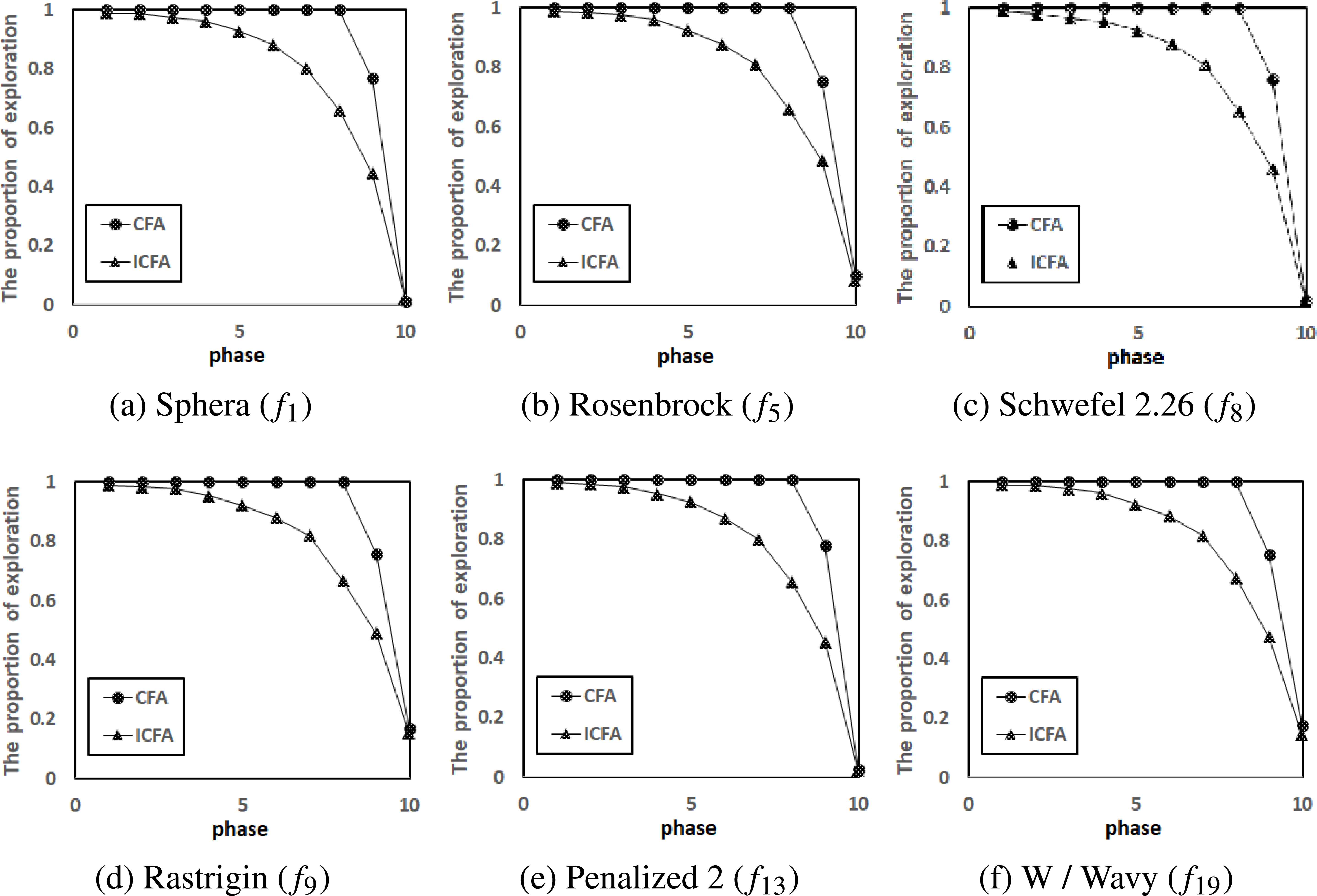
The proportion of exploration in different phases of the CFA and ICFA for the selected benchmark functions with 30 variables.
6. Conclusion
An improved variant of the chaotic firefly algorithm, called ICFA, is proposed in this paper. It was noticed that the FA search equation can be overly random in the beginning of the search process due to the usage of different values of its randomization term for each solution variable. To overcome this issue, a modified movement strategy is proposed to enhance the exploitation ability of the firefly algorithm in the initial generations of a search. Also, the ICFA uses different boundary constraint-handling method in comparison with the FA in order to help maintain diversity in the population.
The effectiveness of the proposed algorithm was investigated on 19 high-dimensional benchmark functions. Three comprehensive experiments are considered in the test design. Experimental results of the first experiment confirmed that the usage of the proposed operator in the first ten percent of the maximum iterations significantly contributes in achieving the superior performance of the proposed ICFA. The findings of the second experiment showed that the proposed ICFA performs better than the standard FA, CFA, and the four recent FA approaches with respect to the accuracy of the results with improved convergence speed. The Wilcoxon’s test with the significance level of 0.05 was employed in order to statistically analyse the performance of the ICFA. The obtained results verify that the performance of the ICFA was statistically better than the FA, CFA and other four FA approaches in the majority of test functions. The results of the third experiment demonstrated that the usage of the proposed modified search strategy enhances exploitation ability of the CFA. Our future study will be focused on developing a new algorithm which would combine the FA with some other popular metahuristic methods in order to solve more complex high-dimensional problems.
Acknowledgments
The second author gratefully acknowledge support from the Research Project 174013 of the Serbian Ministry of Science.
References
Cite this article
TY  - JOUR
AU  - Ivona Brajević
AU  - Predrag Stanimirović
PY  - 2018
DA  - 2018/11/01
TI  - An improved chaotic firefly algorithm for global numerical optimization
JO  - International Journal of Computational Intelligence Systems
SP  - 131
EP  - 148
VL  - 12
IS  - 1
SN  - 1875-6883
UR  - https://doi.org/10.2991/ijcis.2018.25905187
DO  - 10.2991/ijcis.2018.25905187
ID  - Brajević2018
ER  -