
Comparative Study of Basic Time Domain Time-Delay Estimators for Locating Leaks in Pipelines
- DOI
- 10.2991/ijndc.k.200129.001How to use a DOI?
- Keywords
- Cross-correlation; leak detection; leak noise correlator; passive TDE scenario; phase spectrum; time-delay estimation; time-domain methods
- Abstract
The article is devoted to a survey of the known basic Time-Delay Estimation (TDE) methods in the application for detecting fluid leaks in pipeline transport and distribution systems. In the paper, both active and passive estimation methods are considered with respect to the presented generalized classification. However, the main attention is paid to the study of passive methods and their algorithmic implementation. Among the passive methods the Absolute Difference Function (ADF) minimizing algorithms, the Basic Cross-Correlation (BCC) algorithm, the adaptive Least Mean Square (LMS) filtering algorithm are implemented, investigated and compared using a mathematical model of a leak noise signal. All the algorithms are described and the results of the comparison are provided. The advantage of the LMS algorithm in processing the noisy signals is shown. However, its implementation requires choosing a convergence parameter. The necessity in choice of the additional parameter makes the LMS algorithm less practically applicable than the BCC algorithm. The ADF algorithm showed the lowest noise resistivity and can be considered as useful for signal detection, but not for TDE. Some conclusions regarding algorithms’ use for solving the problem of locating leaks are stated. In particular, correlation-based TDE algorithms, as generalized cross-correlation and time-frequency cross-correlation, appear to be the best choice for the implementation of leak detection software.
- Copyright
- © 2020 The Authors. Published by Atlantis Press SARL.
- Open Access
- This is an open access article distributed under the CC BY-NC 4.0 license (http://creativecommons.org/licenses/by-nc/4.0/).
1. INTRODUCTION
The problem of Time-Delay Estimation (TDE) is of great theoretical and practical importance and can be observed in various science and technology fields. The latter is connected with the fact that generally the delay is the time interval between the appearance of some event in one part of the system and its registration in another part of the system. Besides, it is an integral element of dynamic models of physical, chemical, biological, technical and economic systems [1]. However, TDE applications in radio engineering, hydroacoustics, seismology and, especially, in non-destructive testing [1,2] are in the scope of this paper.
The problem of leak location out of a pipeline under pressure, described in detail in Fuchs and Riehle [3], is normally classified as an application in the field of non-destructive testing. The significance of the presented task is beyond any doubt and is due to both the colossal volume of pipelines in operation, and the impossibility of infrastructure’s continuous updating.
The physical basis of the method of determining the leak position is the receiving and processing of an acoustic signal emitted by the leak to the pipe. Remote sensors, located on both sides of the supposed leak, register this signal. However, because the signal is propagated in both directions at the same speed, the time delay between the measured signals on each side of the pipe section can be used to determine the position of the leak, using
Currently, a significant number of methods and algorithms of Digital Signal Processing (DSP) have been developed to solve the TDE problem. Active and passive classes of TDE methods could be distinguished depending on the specifics of the problem being solved [4]. Active methods, in contrast to passive ones, suggest the possibility of emitting a specific special signal in a dynamic system. The parameters of the signal are assumed to be determined a priori. Although the paper focuses on the study of passive TDE methods [3] used to locate leaks, active methods are also briefly discussed in the subsequent section. The discussion is essential for a better understanding of the peculiarities and algorithmic implementation of the passive methods [5,6].
2. CLASSIFICATION OF TDE METHODS
In this section, some well-known TDE methods for various passive and active scenarios are discussed, and their classification is presented. As noted earlier, TDE methods can be divided into active and passive according to their field of use and the mathematical problem statement.
2.1. Passive and Active TDE Scenarios
The generalized TDE task definition is described by the expression [4]
The task of active TDE takes place under conditions of nA(t) = 0 and WA(p) = 1 [4]. In the observed case, Eq. (1) will take the form of
Non-random signal u(t) is a priori known and is called the reference signal. Otherwise, if signal u(t) is not a priori available, the passive TDE problem takes place [7].
It is notable that for locating leaks and some other practical applications it is possible to use an intruder seismic detection. In this case the source of the signal u(t) is within the system. At the same time the impossibility of receiving the signal, generated directly by the object in the system, is assumed [8] to be an active TDE scenario.
2.2. Main Classes of TDE Methods
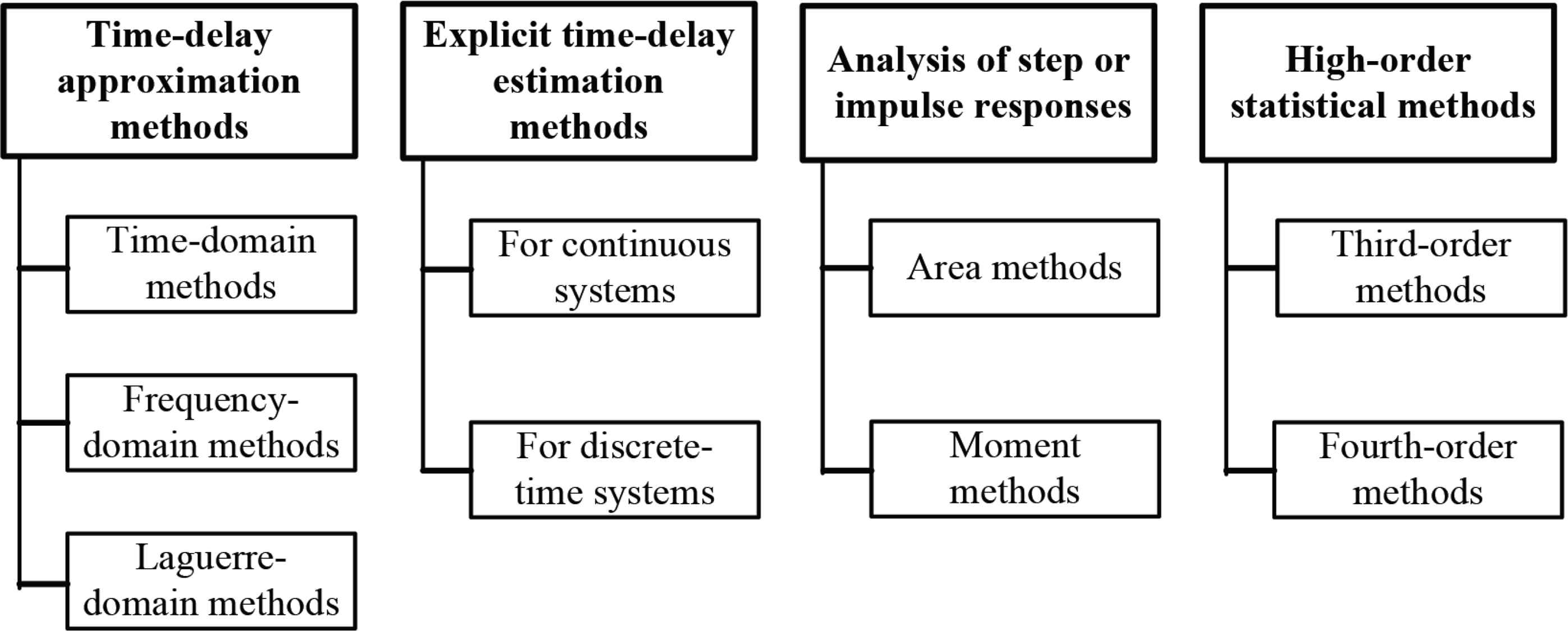
Various approaches and algorithms based on them can be applied to solve the TDE problem. Thus, as it is presented in Björklund [4], TDE methods can be divided into the following groups:
- •
Time-delay approximation methods;
- •
Explicit time-delay estimation methods;
- •
Area and moment statistics methods.
The features, advantages and disadvantages of the described classes of methods are summarized in Table 1. Figure 1 shows a more detailed classification of TDE methods [4].
| Class | Description and Features | ||
|---|---|---|---|
| Theoretical basis | Advantages | Disadvantages | |
| Time-delay approximation methods | Methods are based on the comparison and analysis of signals yA(t) and yB(t), represented in the time-domain or frequency-domain. It is not directly a parameter of a formalized object model.
|
No a priori information about the object is required. | The accuracy of the estimate is strongly influenced by noise. |
| Applicable to passive and active scenarios. | The choice of an efficient approximation algorithm is determined by the task. | ||
| Explicit TDE methods | Methods involve the determination of the
|
Most effective in identifying objects with a time delay. | Methods are active and require a priori knowledge of the object. |
| Designed only for objects of the first, second and third order. | |||
| Area, moment and statistical methods | Methods are based on the established relationship between the type of transient response s(t) of the system or its impulse response and the
|
Allow suppressing random noises with symmetric probability density. | Difficult to implement since they require to define s(t) or h(t). |
Classes of TDE methods
Classes of TDE methods
Methods belonging to the first class, especially time-domain [3,8–10] and frequency-domain [10,11], are widely used to solve the problem of the leak location. The methods presented in other groups are more related to the problem of identifying dynamic objects and are used in control science [4]. The methods, including high-order ones, based on the analysis of the system step response or impulse response are also active [1].
Based on the current practice of locating leaks [3,12], all the TDE algorithms can also be provisionally classified into two groups—correlation-based and non-correlation-based. Both frequency and time methods can be classified within the first group, while most of the non-correlation methods can be considered as time-domain.
3. IMPLEMENTATION OF BASIC TIME DOMAIN TDE METHODS
For further comparison, descriptions and algorithmic implementations of three different time-domain TDE methods are presented. All three considered methods are passive [9] and are suitable for the leak locating purposes. These methods are considered to be the basic [8,9]. Although algorithms used in locating actual leaks are more complex, they have their advantages and disadvantages.
It should be noted that averaging over segments is used to improve the analysis accuracy by increasing the amount of input data [13]. The total number N0 of ticks available in sampled signals is given by
3.1. ADF Minimizing Algorithm
One of the simplest time-domain methods is the non-correlation method of minimizing an Absolute Difference Function (ADF) [8]. The scheme of the method is presented in Figure 2. The following notations are used to describe the algorithms: sA(ti), sB(ti) are the analyzed signals represented by a series of sampled values; TD is the block of the signal time delay for time τj, q is the index of the data segment. Being discrete, ti and τj are multiples of sampling interval Δt
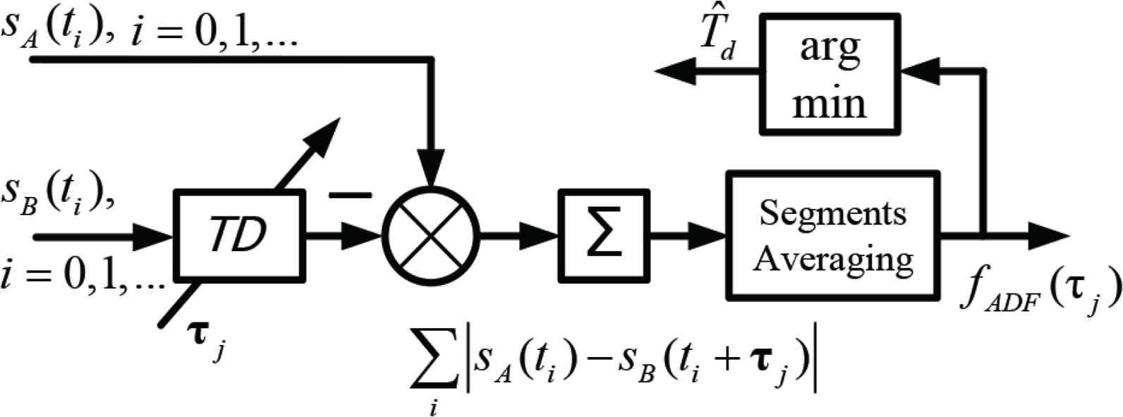
Scheme of TDE via minimizing ADF
The TDA algorithm implies minimization of the difference function between the channel signals shifted in time as follows:
The advantage of this method is computational simplicity and high efficiency of signal detection, but not an optimal estimate of the delay time, especially when the signal is very noisy or distorted [4].
At the same time, the implementation of more complex but similar methods based on the selection of several signals parameters in addition to time delay requires complex calculations. Moreover, the lack of a priori information about the pipeline condition and configuration normally does not allow choosing the proper optimization parameters, which not only affects the locating accuracy but also makes such approximations methods inapplicable at all [14,15].
3.2. BCC Algorithm
Methods based on the calculation and analysis of the cross-correlation function have gained widespread recognition among time-domain TDE algorithms [7]. The procedure is based on the determination of the correlation coefficient between the channels signals, one of which is time-shifted [8]. A simple Basic Cross-Correlation (BCC) TDE scheme [16] is presented in Figure 3.
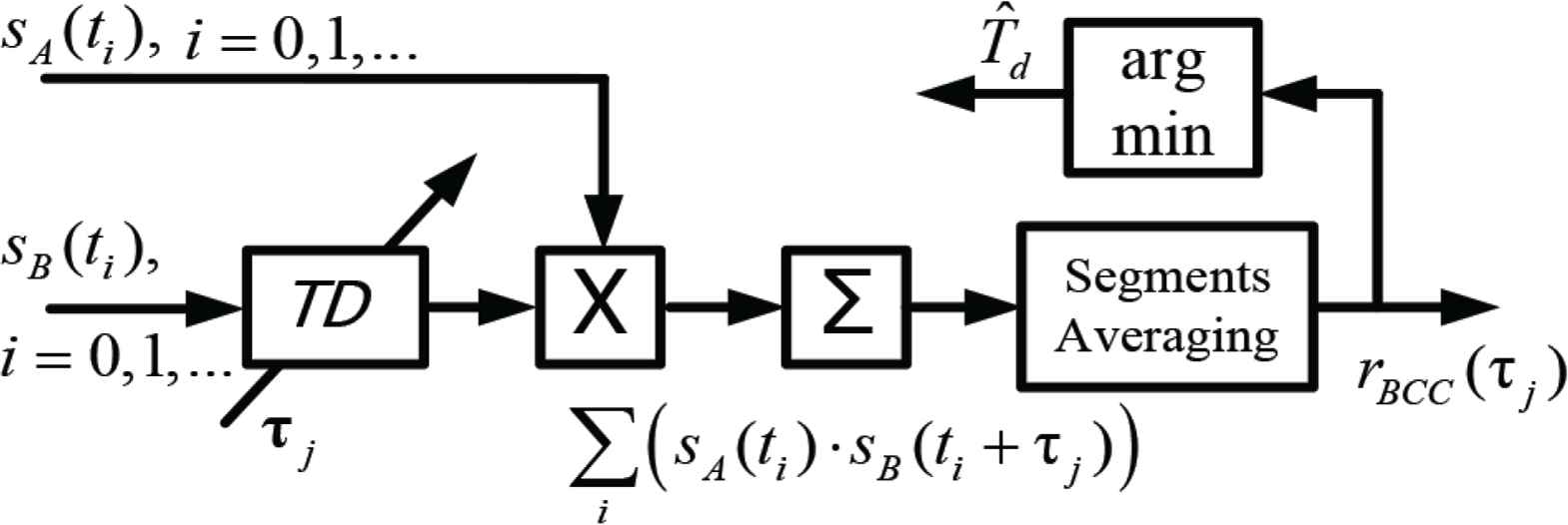
Scheme of TDE via BCC
The algorithm shown in the scheme above is given by
Despite the obvious similarity between Eqs. (3) and (4), their application features differ significantly. Calculations in Eq. (4) require performing only operations of additions and in the absence of high accuracy requirements, can be effectively performed by most computing devices, including microprocessors [17,18]. The efficient calculations require a hardware implementation of the multiplication block with accumulation (multiplier-accumulator). This type of circuit is traditionally considered to be a DSP specific attribute [19].
A more effective correlation method implementation for TDE is the use of generalized cross-correlation algorithms. It differs from the described BCC algorithm by preprocessing [20] of the signals on inputs of the correlator. At the moment, the generalized correlation analysis is considered as the main tool for the acoustic method of locating leaks [10,21].
3.3. Algorithm with the Adaptive LMS Filter
An alternative TDE method [22] is the use of a Finite Impulse Response (FIR) filter. A distinctive feature of the TDE method is the need for iterative refinement of filter coefficients, which makes this solution adaptive. In this case, the resulting solution is for minimizing the root-mean-square error [22,23].
The TDE scheme demonstrating the use of an adaptive filter is presented in Figure 4.
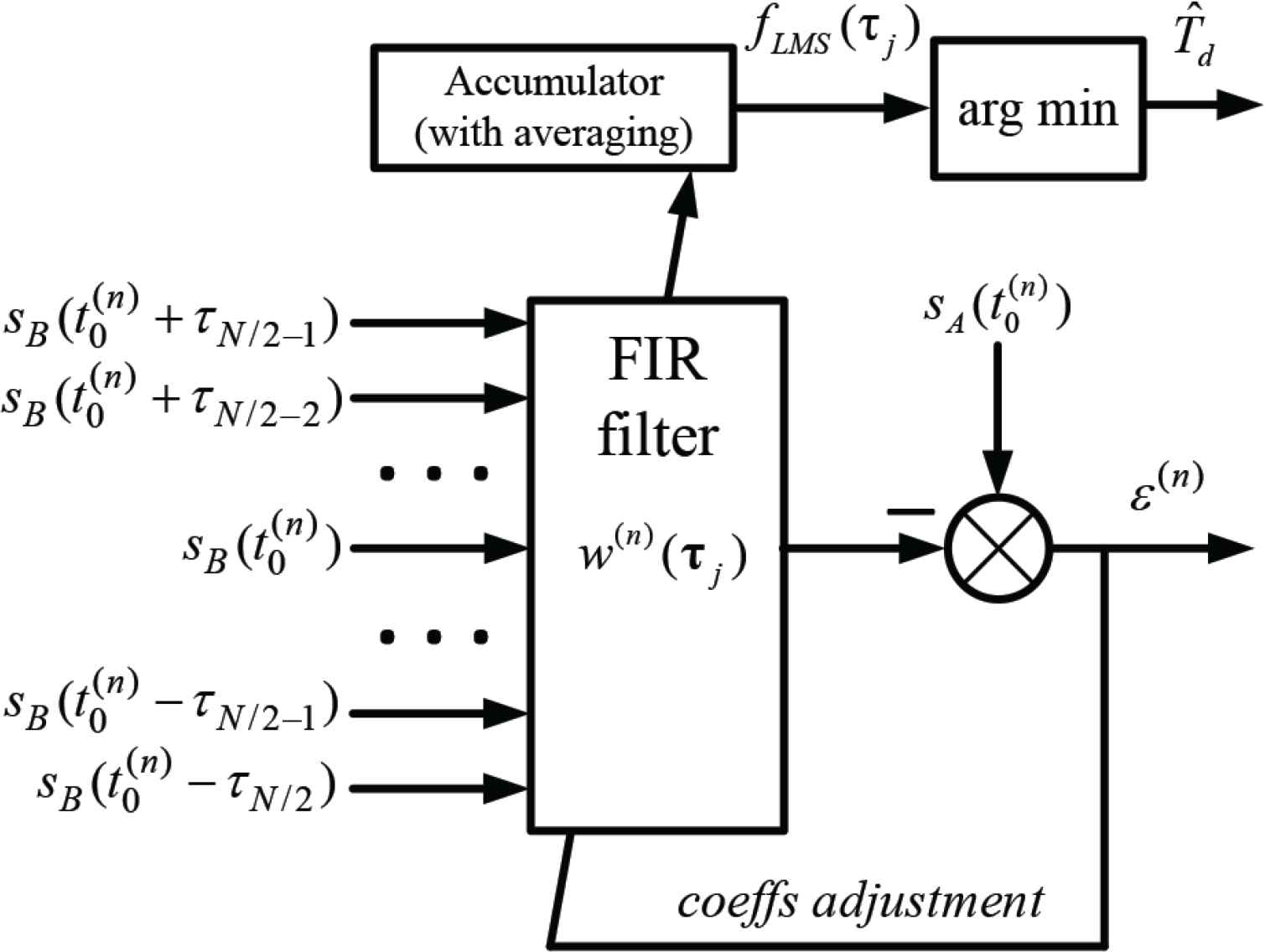
Scheme of TDE with the adaptive LMS filter
The algorithm with the adaptive Least Mean Square (LMS) filter is given by [23]
In Eq. (5) the following notations are used: w(n) (τj) are FIR coefficients of the filter at the nth iteration; ε(n) is error at the nth iteration;
The lag time is estimated by analyzing the FIR filter coefficients after their preliminary averaging
Let us note that, assuming convergence (5), it is worth choosing coefficients kn in (6) in such a way that
The algorithm distinctive feature is applicability and flexibility concerning the amount of input data. In particular, (5) allows processing any amount of newly received data without accumulating N samples in the buffer. The number of necessary iterations is determined by convergence factor μ. To ensure the comparability in the number of computational operations among studied algorithms given by Eqs. (3) and (4), the following assumption was made
3.4. Features of Frequency-Domain TDE
It is known that the temporal and frequency representations of the signal are equivalent in terms of information content [24]. The information about the time lag can be obtained in the frequency domain by determining the phase shift between channel signals [25,26].
From the perspective of the algorithmic implementation, phase response analysis is a complex task, various solutions of which are proposed in Piersol [11], Zhen, and Zi-qiang [24], and Terentiev and Firsov [27]. The algorithmic implementation and comparison of various approaches to TDE based on analysis of the shape of the phase curve are the subject of a separate study and are not considered in this paper.
4. RESULTS AND DISCUSSION
The series of simulations were conducted to compare the ADF, BCC and LMS filtering algorithms for locating pipeline leaks. Signals were generated by software using the leak noise model described further in the corresponding subsection.
In the prospective study N was taken to be consistently equal to 1024, 2048, 4096 and 8192, Q was taken to be 5 in all cases presented below. The values of N and Q were chosen both to utilize the realistic size of the leak noise samples [27] and to provide clear results of the comparison. The sampling interval was assumed to be 44100 Hz.
4.1. Leak Noise Model
The leak noise model is based on the models of additive noise emission [28] and sound propagation along a pipe [29], respectively. According to Brennan et al. [29], to simulate the leak noise signals received by the sensors, the uniformly distributed noise-like signal was processed by pipe filters with dynamic characteristics HA,B ( f, dA,B) given by
The amplitude–frequency response (AFR) of the noise-free test signals is shown in Figure 5. The scale of the graphs along the vertical axis is normalized by the maximum values.
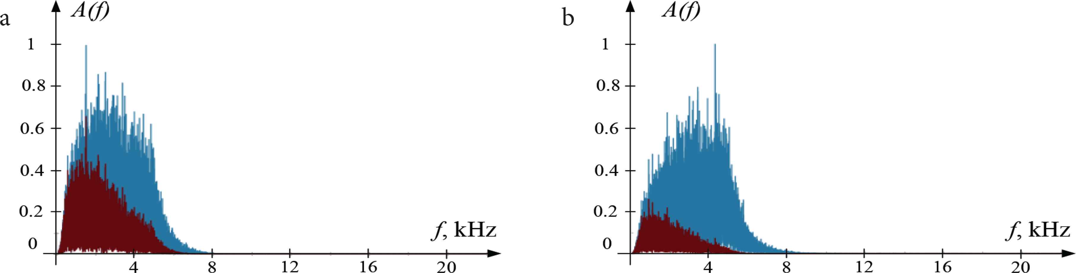
Amplitude–frequency response of test signals (channel A is in red, channel B is in blue). The model of the water supply steel pipe with a mean radius of 84 mm and a wall thickness of 4 mm is used: (a) distances to sensors A and B are 18 and 11 m, respectively; (b) distances to sensors A and B are 22 and 7 m, respectively
The additive noise corrupting the leak noise signal is based on empirical results presented in Papastefanou et al. [28]. Figure 6 shows both AFR and the amplitude envelope of the synthesized noise signals. The intensity of the noise superimposed on the test signals was determined by the target Signal-to-Noise Ratio (SNR). In determining the SNR, the channel with higher intensity of the noise-free signal was taken into account. However, the noise of an identical intensity was superimposed on each of the channels.
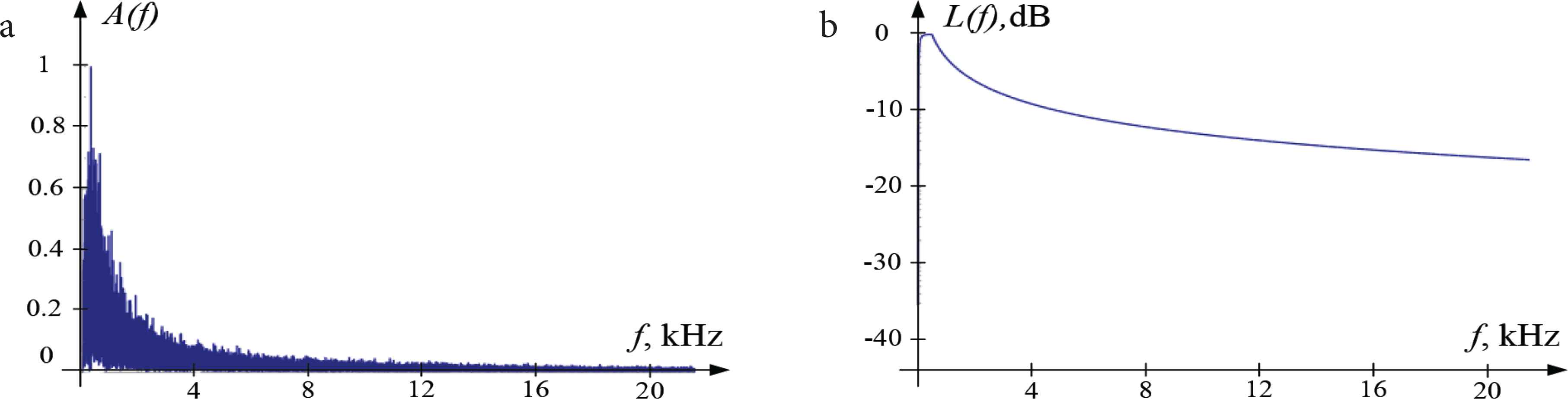
Spectral characteristics of additive noise signals: (a) AFR and (b) amplitude envelope in logarithmic scales
Let us note that the featured leak noise model has its limitations. First, it is not accurate for metal pipes because it is based on the pipe filter that is developed mostly for plastic pipes [29]. Second, the model does not take into account the impact of cavitation [27] and some other effects on emitted acoustic signals. However, the model qualitatively simulates leak noise signals and is relevant for using in the comparative study of the TDE methods. Faerman and Tsavnin [30] discusses the use of the leak noise model and its limitations in more detail.
4.2. Comparison of TDE Algorithms
To compare the ADF, BCC and LMS filtering algorithms, peak-to-mean values were used, which were SNR estimates of the signals at the output of the TDE device [31], calculated according to
TDE error was evaluated according to the formula
Functions at the output of TDE devices for different N and SNR are in Figs. 7 and 8. The scale of the graphs along the vertical axis is maximized.
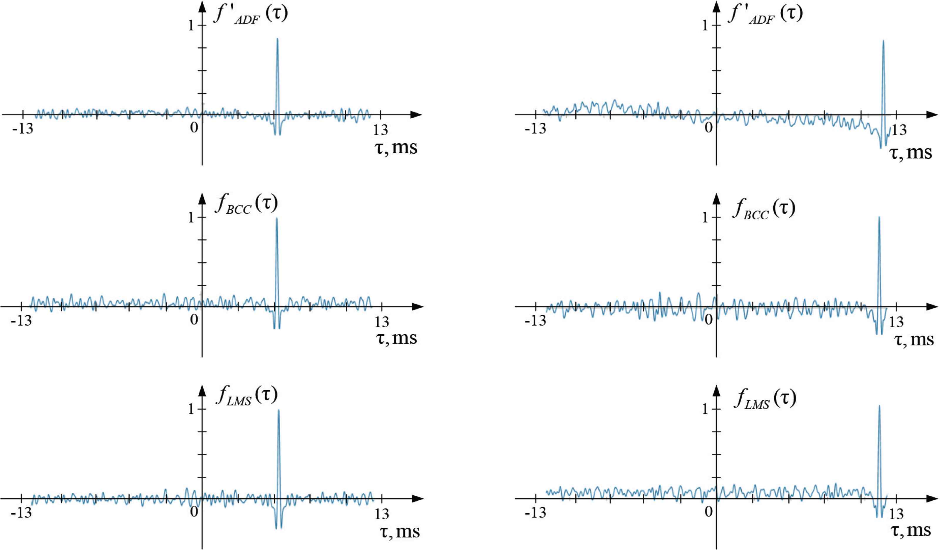
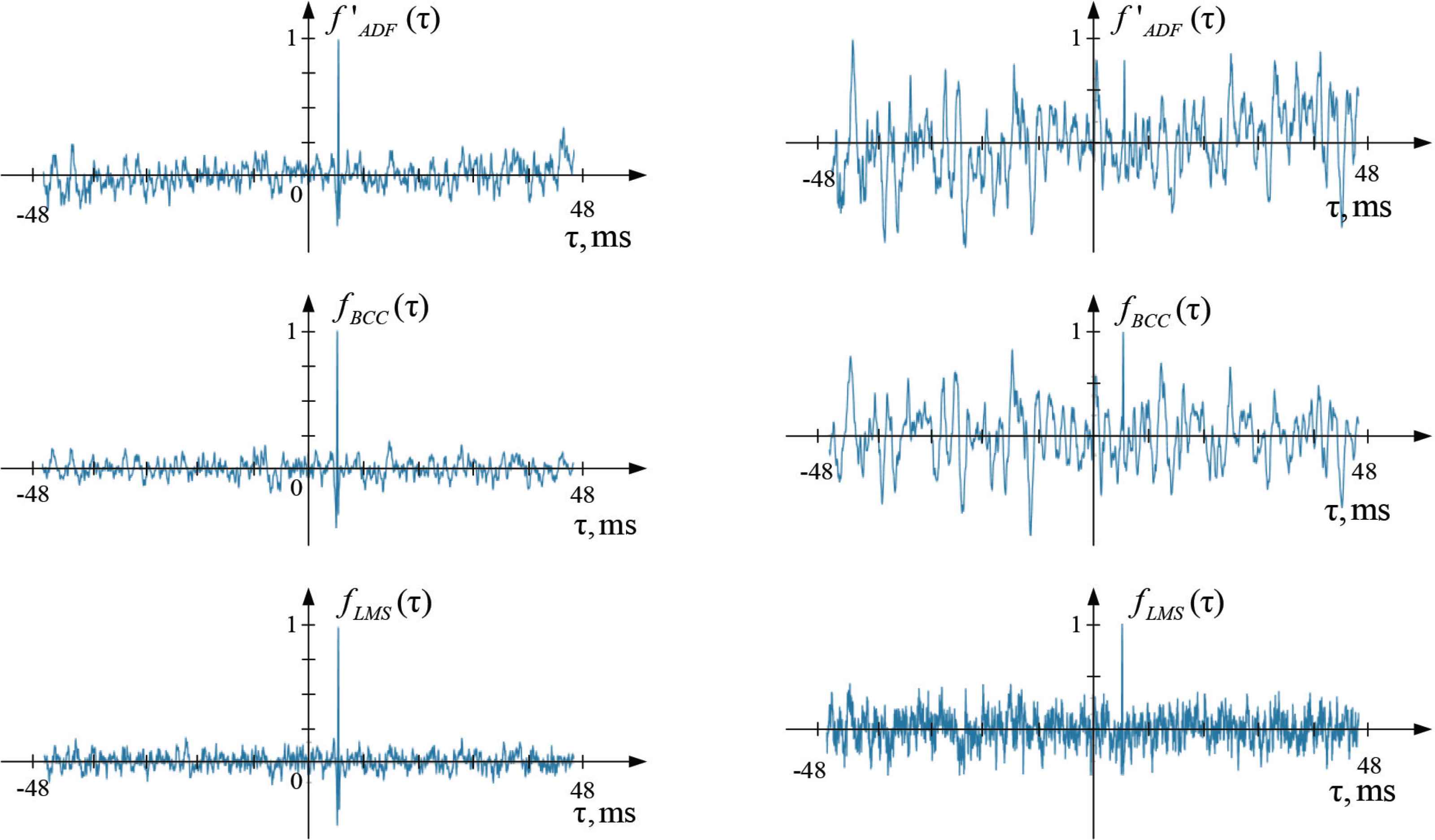
TDE output signals. On the left: signal A, N = 4096, SNR = 1. On the right: signal A, N = 4096, SNR = 0.4
The results of the experiments for different N and SNR are summarized in Tables 2 and 3. In both tables, a single asterisk “*” marks the results where the maximum value at the TDE output is due to the noise influence. A double asterisk “**” marks the results where the detected true maximum of the function is not the only one and there are false peaks of the comparable magnitude.
| SNR | N | ADF TDE | BCC TDE | LMS TDE | |||
|---|---|---|---|---|---|---|---|
| Err (ms) | IADF | Err (ms) | IBCC | Err (ms) | ILMS | ||
| Inf | 1024 | <0.023 | 13.905 | <0.023 | 12.303 | <0.023 | 11.909 |
| 2048 | <0.023 | 18.842 | <0.023 | 17.648 | <0.023 | 16.754 | |
| 4096 | <0.023 | 25.924 | <0.023 | 25.161 | <0.023 | 23.943 | |
| 8192 | <0.023 | 37.883 | <0.023 | 35.536 | <0.023 | 34.024 | |
| 5 | 1024 | <0.023 | 13.610 | <0.023 | 12.149 | <0.023 | 11.675 |
| 2048 | <0.023 | 18.471 | <0.023 | 17.446 | <0.023 | 16.547 | |
| 4096 | <0.023 | 25.505 | <0.023 | 24.849 | <0.023 | 23.658 | |
| 8192 | <0.023 | 36.825 | <0.023 | 35.249 | <0.023 | 33.593 | |
| 2 | 1024 | <0.023 | 11.687 | <0.023 | 10.742 | <0.023 | 10.968 |
| 2048 | <0.023 | 15.592 | <0.023 | 15.747 | <0.023 | 15.153 | |
| 4096 | <0.023 | 20.514 | <0.023 | 20.950 | <0.023 | 22.543 | |
| 8192 | <0.023 | 31.492 | <0.023 | 32.380 | <0.023 | 29.339 | |
| 1 | 1024 | <0.023 | 5.057 | <0.023 | 5.560 | <0.023 | 7.024 |
| 2048 | <0.023 | 6.202 | <0.023 | 8.093 | <0.023 | 10.629 | |
| 4096 | <0.023 | 11.370 | <0.023 | 15.901 | <0.023 | 13.640 | |
| 8192 | <0.023 | 17.993 | <0.023 | 21.558 | <0.023 | 22.937 | |
| 0.4 | 1024 | 12.228* | 2.317 | 2.566* | 3.974 | <0.023** | 3.885 |
| 2048 | 11.809* | 2.683 | <0.023** | 2.758 | <0.023 | 5.506 | |
| 4096 | 27.647* | 2.655 | 3.089* | 3.583 | <0.023 | 6.846 | |
| 8192 | 76.105* | 3.798 | <0.023** | 3.171 | <0.023 | 9.575 | |
Results of TDE for various sizes of data segment (signal in Figure 5a)
| SNR | N | ADF TDE | BCC TDE | LMS TDE | |||
|---|---|---|---|---|---|---|---|
| Err (ms) | IADF | Err (ms) | IBCC | Err (ms) | ILMS | ||
| Inf | 1024 | <0.023 | 12.554 | <0.023 | 11.457 | <0.023 | 10.292 |
| 2048 | <0.023 | 15.053 | <0.023 | 17.560 | <0.023 | 15.521 | |
| 4096 | <0.023 | 20.115 | <0.023 | 25.276 | <0.023 | 22.754 | |
| 8192 | <0.023 | 29.649 | <0.023 | < 0.023 | <0.023 | 33.172 | |
| 5 | 1024 | <0.023 | 11.147 | <0.023 | 10.389 | <0.023 | 9.867 |
| 2048 | <0.023 | 13.684 | <0.023 | 16.624 | <0.023 | 14.731 | |
| 4096 | <0.023 | 18.241 | <0.023 | 24.326 | <0.023 | 21.703 | |
| 8192 | <0.023 | 27.883 | <0.023 | 34.698 | <0.023 | 31.583 | |
| 2 | 1024 | <0.023 | 6.056 | <0.023 | 5.875 | <0.023 | 8.072 |
| 2048 | <0.023 | 10.054 | <0.023 | 11.058 | <0.023 | 10.816 | |
| 4096 | <0.023 | 14.912 | <0.023 | 17.193 | <0.023 | 15.961 | |
| 8192 | <0.023 | 21.406 | <0.023 | 25.120 | <0.023 | 22.287 | |
| 1 | 1024 | 18.569* | 2.322 | 9.458* | 2.562 | <0.023 | 4.911 |
| 2048 | 18.823* | 3.050 | 18.846* | 3.841 | <0.023 | 6.155 | |
| 4096 | <0.023 | 3.755** | <0.023 | 4.796 | <0.023 | 8.335 | |
| 8192 | <0.023 | 6.836 | <0.023 | 9.991 | <0.023 | 11.435 | |
| 0.4 | 1024 | 22.383* | 2.370 | 10.637* | 2.472 | 22.587* | 4.296 |
| 2048 | 10.451* | 2.711 | 7.871* | 2.449 | 20.819* | 3.178 | |
| 4096 | 50.796* | 2.890 | 13.426* | 2.826 | <0.023 | 4.852 | |
| 8192 | 74.265* | 3.030 | 74.515* | 3.566 | <0.023 | 4.484** | |
Results of TDE for various sizes of data segment (signal in Figure 5b)
4.3. Outcomes and Prospects
The dependences of the SNR signals at the output of estimators on N (Figure 9) and on the SNR of the input signals are constructed based on the study (Figure 10).
Peak-to-mean ratio of the estimator’s output signal (a) linear scaling of the independent variable; (b) square root scaling of the independent variable.
Peak-to-mean ratio of the estimator’s output signal (curves are smoothed)
Equations (7)–(9) show that the following ratio takes place
At the same time, any values of I (N, f ) < 4 can be considered equivalent based on the results of the study. They typically indicate that an unambiguous TDE by the peak value of the function is impossible.
Similarly, any values of I (N, f ) > 8 can be considered equivalent for the opposite reason. The change in I (N, f ) in the range from 4 to 8 is further considered as a metric for evaluating the influence of noise on the compared methods. The general character of empirical dependence
The dependence in Figure 10 allows establishing the advantage of the LMS method comparing the mutual position of the curves in region 4 < I (N, f ) < 8.
The main outcomes of the comparison are as follows:
- •
implementation of the ADF minimizing algorithm is simple and does not require multiplication operations. The disadvantage is the high noise sensitivity which limits the practical application of the algorithm;
- •
the BCC algorithm is distinguished by relatively good noise resistivity and presence of efficient computational schemes realized via the fast Fourier transforms;
- •
the TDE method using an adaptive LMS filter has a high noise resistance and flexibility in respect to the size of the input data. These advantages make the method applicable in the absence of a priori information about the signals. At the same time, ensuring convergence requires solving the additional problem of choosing parameter μ.
It is notable that for implementation of correlation TDE methods the convolution theorem [16] is normally used instead of Eq. (4). This measure provides better processing time for all N > 128 [16].
The correlation methods applicability potential is also determined by the possibility of using the generalized cross-correlation algorithms, which in most cases can increase the accuracy of TDE [10,21] without a significant increase in computational complexity.
Another modification of correlation TDE methods is the time-frequency correlation analysis described in Ref. [32]. The advantage of the time-frequency approach is the ability to display visually both the frequency and time features of the analyzed signals [33]. The use of the time-frequency correlation method in leaks detection makes the correlation peaks more clear and the analysis more informative [32,33].
5. CONCLUSION
In the paper, the basic classes of TDE methods have been investigated, and some basic time-domain correlation and non-correlation algorithms have been compared with reference to the particular problem of determining the pipeline leak location.
In respect to the presented classification of TDE methods, a variety of methods was discussed. Among the class of passive TDE approximation methods, three basic algorithms were compared. All the algorithms with data segmentation and averaging were proposed and described in detail.
Comparative study of the algorithms was performed on model-generated signals. The leak noise model is based on noise-like signals which were applied to pipe filters. Despite the discussed limitations of the model, it is applicable for qualitative simulation of the leak noise.
The comparison was based on formal criteria of measuring the information value of the TDE functions as well as on the accuracy of estimation. Peak-to-mean values were considered to be a quantitative measure of the function’s information value. The proposed criteria have proved to be relevant for formal comparison of TDE.
The performance of three TDE algorithms was studied for various SNR and sizes of data segments. The ADF minimizing algorithm shows the lowest noise tolerance and should not be used for processing noisy signals. However, for signals with decent SNR, the ADF minimizing algorithm shows results that are comparable to other TDE algorithms under study.
Some advantages of correlation algorithms were stated, in particular, satisfactory resistance to the random noise influence, computational efficiency, and implementation simplicity. At the same time, despite the complexity of the practical application, the LMS TDE method has proved efficient in dealing with intense additive noises.
CONFLICTS OF INTEREST
The authors declare they have no conflicts of interest.
REFERENCES
Cite this article
TY  - JOUR
AU  - Vladimir A. Faerman
AU  - Valeriy S. Avramchuk
PY  - 2020
DA  - 2020/03/18
TI  - Comparative Study of Basic Time Domain Time-Delay Estimators for Locating Leaks in Pipelines
JO  - International Journal of Networked and Distributed Computing
SP  - 49
EP  - 57
VL  - 8
IS  - 2
SN  - 2211-7946
UR  - https://doi.org/10.2991/ijndc.k.200129.001
DO  - 10.2991/ijndc.k.200129.001
ID  - Faerman2020
ER  -