1. INTRODUCTION

Nowadays, operating systems have become more complex and more efficient due to the multitasking functionality, which allows several processes to run simultaneously. The Operating System (OS) chooses a task from the Ready Queue (RQ) and allocates it to a processor, this process is known as scheduling. When several processes are in the RQ, the OS plays an important role in choosing the correct order of execution of the processes for achieving better Average Turnaround Time (ATAT) and Average Waiting Time (AWT). Task scheduling algorithms can also be applied in the cloud-computing environment; it is one of the most important activities in this environment.

First-Come-First-Serve (FCFS), Shortest Job First (SJF), Min–Min, Max–Min are examples of task scheduling algorithms. In FCFS, a task that comes first executes first [1]. In this algorithm, no priority is supported. While in the SJF algorithm, the tasks with a minimum execution time will have priority to be executed [2]. In the Min–Min algorithm, smaller tasks are selected to be executed first; on the other hand, Max–Min algorithm selects the bigger tasks to be executed first [3].

Among the most well-known existing scheduling algorithms the Round Robin (RR) algorithm, because it is suitable for job scheduling in time-sharing systems due to its simplicity, fairness and generality. In Round Robin, the tasks are distributed based on the arrival time (First In, First Out way) but with a limited CPU time called “quantum”. If a process does not complete before its quantum expires, the quantum is passed to the next pending process in the queue, and the uncompleted process is placed at the end of the ready processes queue. The algorithm will run again until all the tasks are executed [2].

Round Robin algorithms are categorized into two types; Static RR and Dynamic RR (DRR). In static RR, a time quantum is determined at the beginning of the task scheduling and remains until the end. This algorithm has several drawbacks due to the fixed choice of the quantum. If the quantum is large, the tasks having a high execution time can occupy the processor for a long time and the small tasks remain to wait, and if the quantum is small, tasks with a high execution time take a long time to be executed. Contrary to RR with a variable quantum, that automatically adjusts to tasks in the queue. Although the existing approaches using a dynamic time quantum do not use multi parameters in the choice of the quantum, which affect the process of scheduling and the performances of the system.

In this paper, we present an improved version of Round Robin with varying time quantum. The main contributions of our work can be summarized as follows:

1. (i)

   Proposes an analytical model that takes into consideration different parameters to determine the order of tasks execution. The use of burst time as parameters in our model ensures a more suitable time quantum.

2. (ii)

   Reduce the average turnaround time ATAT and the average waiting time AWT of existing tasks, which leads to a better use of resources that is considered as one of the major problems in the operating system and cloud computing environment.

3. (iii)

   The performance of the proposed algorithm has been analysed through five cases studies and compared with traditional RR, AN Improved Round Robin CPU Scheduling Algorithm With Varying Time Quantum (IRRVQ), An efficient Average Execution Time-RR (AET-RR) scheduling algorithm and Tajwar et al. [4].

For this purpose, this paper is organized as follows. Section 2 focuses on some related works. In Section 3, the proposed approach is presented in detail. Section 4 contains the proposed approach results and discussions. Finally, we conclude our work and describe future works in Section 5.

2. RELATED WORKS

In the past few years, several works have been carried out to optimize the task scheduling process. In this section, we will quote the works most related to our problematic.

The authors of Lin et al. [5] presented a new algorithm for energy-aware virtual machine scheduling and consolidation, called DRR. Eucalyptus [6] is used to show the comparison between the proposed algorithms, GREEDY, ROUNDROBIN and POWERSAVE in terms of economy of the physical machines used and energy consumption. The DRR shows his superiority compared to the traditional Round Robin. Compared to POWERSAVE scheduling, the proposed algorithm requires fewer physical machines and consumes less power.

Kumar Mishra and Rashid proposed AN Improved Round Robin CPU Scheduling Algorithm With Varying Time Quantum (IRRVQ). In this algorithm, the features of SJF and RR scheduling algorithms are combined with varying time quantum. Initially, the processes in the ready queue are arranged in the ascending order of their burst time. CPU is allocated to the first process in the ready queue and time quantum is put equal to his burst time. Processes are arranged in the ascending order after each cycle; the operation is repeated until the ready queue is empty. Compared to traditional RR scheduling algorithm, the IRRVQ showed his superiority in reducing the waiting time and turnaround time. Although the IRRVQ scheduling algorithm does not take into consideration if the task is heavy or light, this can lead to an important waiting time [7].

Dash and Samantra presented a new CPU scheduling algorithm that use dynamic time quantum named as dynamic average burst round robin. By minimizing the average waiting time and average turnaround time, the proposed algorithm provides better performance metrics than traditional Round Robin, Dynamic Quantum with Re-adjusted Round Robin (DQRRR), IRRVQ, Self-Adjustment Round Robin (SARR), and Modified Round Robin (MRR) [8].

Pradhan et al. [9] presented a MRR algorithm by using dynamic time quantum rather than fixed time quantum. The proposed algorithm is implemented in MATLAB [10] in which the reducing of waiting time and turnaround time is improved compared to traditional RR.

Mohamed et al. [2] presented two dynamic enhanced algorithms of Round Robin: Dynamic Priority Round Robin (DPRR) and Enhanced DPRR (EDPRR), to eliminate the disadvantages of fixed quantum. The DPRR algorithm calculates a dynamic time quantum depending on the processing time of tasks. In the second algorithm (EDPRR), the tasks selected to be executed is based in execution time. The results show that the proposed algorithms achieve high resource utilization and minimize the waiting time and the turnaround time of tasks in cloud computing environment comparing to EPRR.

Singh and Agrawal aimed to create an efficient Round Robin algorithm in the Cloud computing environment. The algorithm is the combination of RR, priority and SJF CPU scheduling algorithm, using a dynamic time quantum. The comparison result shows that the proposed algorithm performs better than RR and subcontrary mean dynamic round robin scheduling algorithm. The goal of the proposed algorithm was achieved by reducing the waiting time, TAT and context switches [11].

Mora and Junaidu presented a modified median round robin algorithm. In this algorithm, a variable time quantum is used to eliminate the drawback of popular RR scheduling algorithms. The research work proves an efficient solution compared to RR, IRR, improved mean round robin with shortest job first scheduling, half life variable quantum time round robin and dynamic round robin with controlled pre-emption in terms of minimizing waiting time, TAT, response time and the Number of Context Switching (NCS). However, the proposed algorithm does not deal with the case of different arrival times and priorities of tasks [12].

Arif and Javed introduced a new scheduling algorithm by using two-time quantum for scheduling the ready queue, which are used alternately in cycles of scheduling. The algorithm gives first priority to reduce the NCSs and waiting time, and second priority to response time. The comparative result with RR, A New Round Robin Based Scheduling Algorithm for Operating Systems (AN), shortest remaining burst round robin Scheduling Algorithm and Modulus-based Round Robin Scheduling Algorithm (MB) show the superiority of proposed algorithm in reducing waiting time, NCSs and response time [13].

Elmougy and Joundy proposed a novel hybrid task-scheduling algorithm named SRDQ (SJF and RR with Dynamic Quantum hybrid algorithm) combining Round Robin (RR) and SJF scheduling algorithms. The SRDQ uses a dynamic variable time quantum. In this algorithm, the ready queue is splitting using the median into two sub-queues: Q1 for short tasks and Q2 for the longer one. Tasks will be executed mutually two short tasks from Q1 and one long task from Q2. The results prove the effectiveness of the proposed algorithm in reducing waiting time, response time and partially the starvation of long tasks compared to traditional RR and SJF algorithms [14].

Dave et al. [15] presented a novel CPU scheduling algorithm using dynamic time quantum. The approach gives more priority to reducing the context switching of process in queue. The simulation result improves the efficiently of the proposed approach.

Tajwar et al. [4] proposed an enhanced round robin algorithm with varying time quantum. The evaluation of the algorithm indicates an improved performance in AWT, ATAT and context switching compared to traditional RR, DQRRR scheduling algorithm, IRRVQ, and self-adjustment-round-robin (SARR).

Sudhansu and Sugyan proposed an AET-RR algorithm for online and offline scenario with varying Time Quantum (TQ). The algorithm is an improvement version of traditional RR. The experimental analysis shows the effectiveness of the proposed algorithm in terms of AWT, ATAT and the NCS compared to the traditional RR algorithm [16].

Several round robin algorithm enhancements have been developed. Some of them have used a fixed TQ that leads to a large waiting time for the tasks in the ready queue. Others have used the dynamic TQ principle, which gives better results. However, the majority of algorithms do not consider the type of task (heavy or light) and their arrival time in the choice of TQ leading to increase the average waiting time and turnaround time, which affects the system performance. So in this paper, we tried to overcomes the limitations of existing solutions by taking into consideration the type of tasks, their arrival time and by proposing an analytical model for sorting the process list for their scheduling.

3. PROPOSED APPROACH

As mentioned before, in this work we proposed an improved version of round robin scheduling algorithm. The choice of time quantum value is a real challenge as if the TQ is too short, too many context switches will lower the CPU efficiency while if it is long, the heavy tasks will busy the processor, which leads to a long average waiting time. So, we focus on the right choice of TQ.

We propose an analytical model for sorting the list of task, the result of the sorted list will determine the choice of TQ. The list is sorted according to the cost of each task CT(i):

α, β weighting coefficients, α + β = 1 i: number of task.

Rarr(Ti): Rate of arrival time of task T(i).

Rbut(Ti): Rate of burst time of task T(i).

Equations (2) and (3) respectively represent the equations of Rarr and Rbut.

Tarr(Ti): arrival time of task T(i).

N: number of tasks in the ready queue.

BT(Ti): burst time of task T(i).

N: number of tasks in the ready queue.

From (1) to (3) the cost function of scheduling tasks in the list is as follows:

Two list cases occur. We can have a list with the zero arrival time and the second case with a variable arrival time. In what follows we present the algorithm of the proposed approach:

1. 1.

   Input initial list of tasks.

2. 2.

   Apply the analytic model that gives a sorted list.

3. 3.

   If the arrival time of all tasks AT = 0.

4. 4.

   If the sorted list is ordered in ascending order of burst time,

   • •

     select the middle value of burst time of sorted list (MBT).

   • •

     divide the ready queue into two sub-lists (light tasks list and heavy tasks list) according to MBT.

   • •

     Execute first the task which is in the light list (with Quantum = burst time of middle task).

   • •

     after, execute tasks which are in the heavy list (with Quantum = burst time of middle task).

5. 5.

   Else execute directly the processes without split them (with Quantum = burst time of middle task).

6. 6.

   Else (If AT ≠ 0)

   • •

     Execute directly the task with Quantum = burst time of first task/2.

   • •

     Check the ready queue; if two or more tasks arrive in the ready queue, apply the analytical model.

7. 7.

   If the sorted list is ordered in ascending order of burst time, go to 4.

8. 8.

   Else, go to 5.

In what follows we present a description of the proposed algorithm. The application result of the analytical model is a list of tasks sorted according to the task cost.

• •

  If the arrival time of all tasks is equal to zero, we apply a dynamic time quantum in each iteration, Using burst time of the middle task we divide the ready queue into two sub-queues: Tasks having burst time less than the middle are stored in the first list (light task list), and the rest of tasks in the second list (heavy task list).

  The tasks in the first queue are executed first following these steps:

  1. (1)

     The CPU is allocated to tasks using RR scheduling with a small-time unit (time quantum) equal to the burst time of the middle task.

  2. (2)

     The process is repeated until the list is empty.

• •

  After all the tasks in the first queue have been executed, the same steps are applied to schedule the tasks of the second list.

• •

  If tasks are arriving in the ready queue at different time:

  1. (1)

     The time quantum value is set equal to the burst time of the first process divided by two.

  2. (2)

     When the first task is executed, we check the new tasks arrived in the queue, we apply them the analytical model to have a new list sorted.

  3. (3)

     If the sorted list is in ascending order of burst time:

     1. (i)

        We divide it into two sub-lists using the algorithm mentioned above.

     2. (ii)

        Else, we execute the tasks by putting the time quantum equal to the burst time of the middle task.

     3. (iii)

        After each execution of a process, we check in the ready queue if a new process has arrived, we update the order of the tasks by applying the analytical model again.

4. RESULTS AND DISCUSSION

In this section, we present the results of the proposed approach on five different cases of list. In order to prove the effectiveness of our approach and to ensure a fair comparison between the proposed approach and the existing algorithms, we opted for examples used in the majority of these algorithms, with the same number of tasks, same burst time and arrival time. The proposed algorithm works with any other examples.

The first and the fourth cases present a list of tasks with zero arrival time; the other cases present a list with variable arrival time. Five processes P1, P2, P3, P4 and P5 have been considered.

4.1. Case 1: Process with Zero Arrival Time

The processes are arriving at time 0 with burst time 105, 60, 120, 48 and 75 respectively. The analytic model is applied to define the new order of tasks, which are P4, P2, P5, P1 and P3.

Using the burst time of the middle process, we divide the ready queue into two sub-queues. The first sub-queue contains the processes P4, P2 and P5, the second one contains P1 and P3.

Initially, the processes of the first sub-queue are executed: The time quantum value is set equal to the burst time of the middle process i.e. 60. CPU is allocated to the processes P4, P2 and P5 for a time quantum of 60 milliseconds (ms). After the first cycle, the burst time of processes P4, P2 and P5 are equal to 0, 0 and 15 respectively. The processes P4 and P2 are finished execution, so they are removed from the ready queue. The time quantum value is set to the burst time of P5 i.e. 15. The CPU is allocated to process P5 for a time quantum of 15 ms. After the second cycle, the burst time of P5 is 0 so the process is removed from the ready queue. The first sub-queue is empty so the second sub-queue begins execution: The time quantum value is set equal to the burst time of the middle process, in this case, we have two processes P1 and P3, so we calculate the average of their burst time, it is equal to 112.5. CPU is allocated to the processes P1 and P3 from the ready queue for a time quantum of 112.5 ms. After the third cycle, the burst time of P1 and P3 are 0 and 7.5 respectively. The process P1 has finished execution, so it is removed from the ready queue. Now only P3 in the ready queue, so CPU is allocated to P3 for a time quantum of 7.5 ms. The waiting time of P1 is 183 ms, for P2 is 48 ms, 288 ms for P3, 0 ms for P4, 108 ms for P5.

Table 1 shows the arrival time and burst time of processes. Figure 1 shows the Gantt chart representation of RR. Figure 2 shows the Gantt chart representation of IRRVQ. Figure 3 shows the Gantt chart representation of Tajwar et al. [4]. Figure 4 shows the Gantt chart representation of the proposed algorithm. The comparison result of RR, IRRVQ, Tajwar et al. [4] and the proposed algorithm is shown in Table 2. Figure 5 shows a graphical comparison of RR, IRRVQ, Tajwar et al. [4] and proposed approach in terms of ATAT and AWT.

Process	Arrival time	Burst time
P1	0	105
P2	0	60
P3	0	120
P4	0	48
P5	0	75

Table 1

Processes with zero arrival time (Case 1)

Figure 1

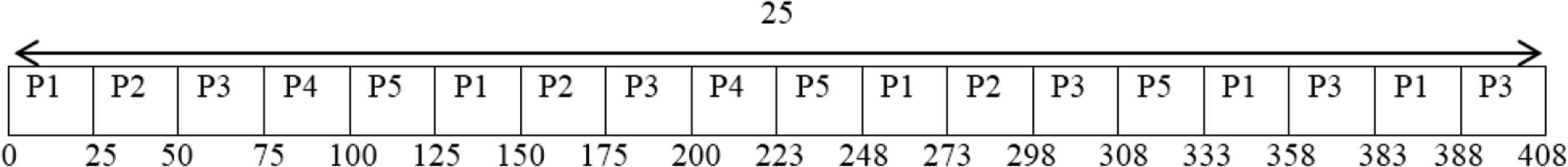
Gantt chart representation of RR with quantum time 25.

Figure 2

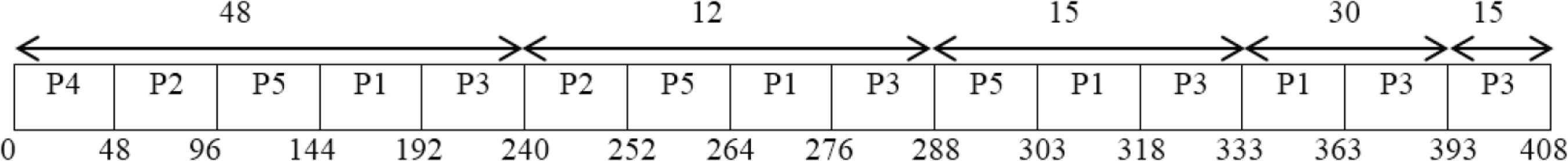
Gantt chart representation of IRRVQ with quantum time 48, 12, 15, 30 and 15.

Figure 3

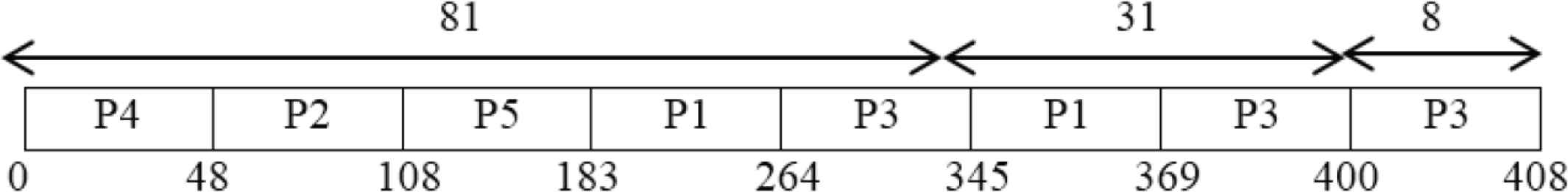
Gantt chart representation of Tajwar et al. [4] with quantum time 81, 31 and 8.

Figure 4

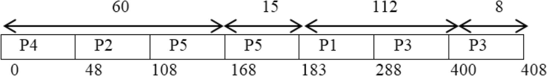
Gantt chart representation of proposed algorithm with quantum time 60, 15, 112 and 8.

Algorithm	Time quantum (TQ)	Waiting time of each process	Average waiting time (ms)	Average turnaround time (ms)
RR	25	P1 = 283, P2 = 223, P3 = 288, P4 = 175, P5 = 258	245.4	327
IRRVQ	48, 12, 15, 30, 15	P1 = 258, P2 = 192, P3 = 288, P4 = 0, P5 = 228	193.2	274.8
Tajwar	81, 31, 8	P1 = 264, P2 = 48, P3 = 288, P4 = 0, P5 = 108	141.6	223.2
Proposed approach	60, 15, 112.5, 7.5	P1 = 183, P2 = 48, P3 = 288, P4 = 0, P5 = 108	125.4	207

Table 2

Comparison results (Case 1)

Figure 5

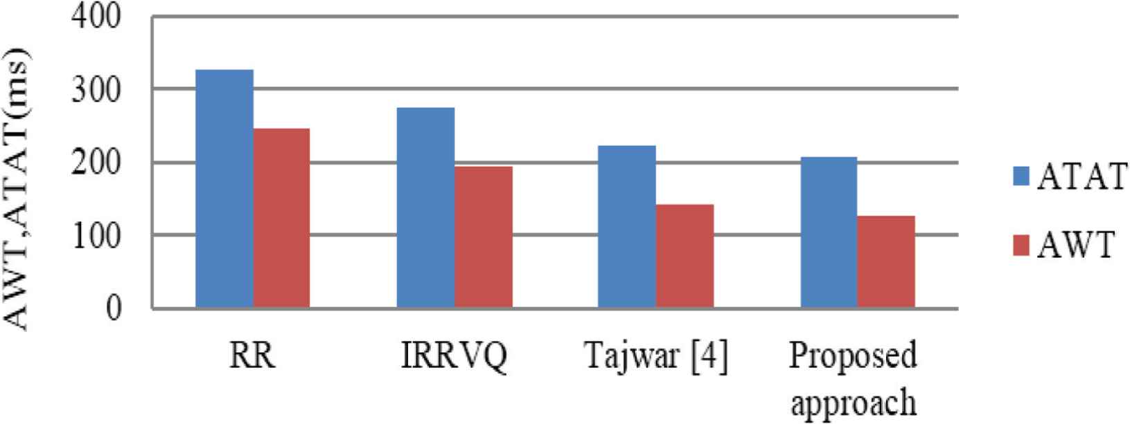
Comparison of RR, IRRVQ, Tajwar et al. [4] and proposed approach by taking ATAT and AWT (Case 1).

With the same number of processes, the same arrival time and burst time:

• •

  The AWT is 125.4 ms in the proposed algorithm, 245.4 ms in RR, 193.2 ms in IRRVQ, and 141.6 ms in Tajwar et al. [4].

• •

  The ATAT is 207 ms in proposed algorithm while ATAT is equal to 327 in RR, 274.8 in IRRVQ and 223.2 in Tajwar et al. [4].

4.2. Case 2: Variable Arrival Time

In this case, processes are arriving at a different time. Five processes P1, P2, P3, P4 and P5 arriving at time 0, 5, 8, 10 and 13 respectively with burst time 20, 45, 15, 4 and 9.

The time quantum value is set equal to the burst time/2 of the first process in the ready queue i.e. 10. CPU is allocated to the process P1 from the ready queue for a time quantum of 10 ms. After the first cycle, the burst time of P1 is 10 and P2–P4 have arrived in the ready queue. The analytic model is applied to define the new order of tasks, which is: P1, P4, P3, and P2. The time quantum value is set equal to the burst time of the middle process in the ready queue i.e. 9.5. CPU is allocated to the processes P1, P4, P3 and P2 for a time quantum of 9.5 ms, after the execution of P1 the process P5 has arrived in the ready queue, so we re-apply the analytic model to the existing tasks, the new order is P1, P4, P3, P5, and P2. The time quantum value is set equal to the burst time of the middle process in the ready queue i.e 15. CPU is allocated to the processes P1, P4, P3, P5 and P2 for a time quantum of 15 ms. After the third cycle, the burst time of processes P1, P4, P3, P5 and P2 are equal to 0, 0, 0, 0 and 30. The CPU is allocated to the only process in the queue P2 for a quantum time of 30 ms.

Table 3 shows the arrival time and burst time of processes. Figure 6 shows the Gantt chart representation of RR. Figure 7 shows the Gantt chart representation of IRRVQ.

Process	Arrival time	Burst time
P1	0	20
P2	5	45
P3	8	15
P4	10	4
P5	13	9

Table 3

Processes with variable arrival time (Case 2)

Figure 6

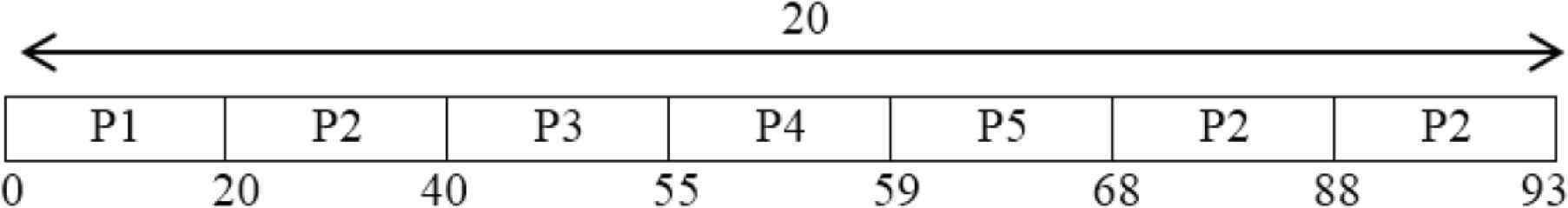
Gantt chart representation of RR with Quantum time 20.

Figure 7

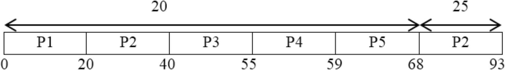
Gantt chart representation of IRRVQ with quantum time 20 and 25 respectively.

Figure 8 shows the Gantt chart representation of Tajwar et al. [4]. Figure 9 shows the Gantt chart representation of the proposed algorithm. The comparison result of RR, IRRVQ, Tajwar et al. [4] and our algorithm is shown in Table 4. Figure 10 shows a graphical comparison of RR, IRRVQ, Tajwar et al. [4] and proposed approach in terms of ATAT and AWT. With the same number of processes and the same arrival time and burst times:

• •

  The average waiting time is 19 (ms) in the proposed algorithm, 33.2 ms in RR, IRRVQ and Tajwar et al. [4].

• •

  The average turnaround time is 37.6 ms in proposed algorithm, 51.8 in RR, in IRRVQ and Tajwar et al. [4].

Figure 8

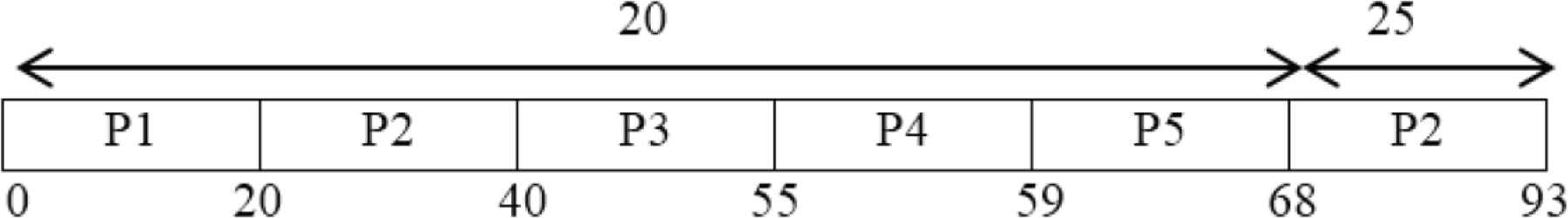
Gantt chart representation of Tajwar et al. [4] with quantum time 20 and 25 respectively.

Figure 9

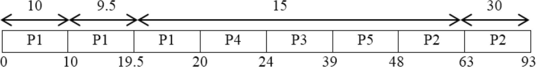
Gantt chart representation of proposed algorithm with quantum time 10, 9.5, 15 and 30.

Algorithm	Time quantum (TQ)	Waiting time of each process	Average waiting time (ms)	Average turnaround time (ms)
RR	20	P1 = 0, P2 = 43, P3 = 32, P4 = 45, P5 = 46	33.2	51.8
IRRVQ	20, 25	P1 = 0, P2 = 43, P3 = 32, P4 = 45, P5 = 46	33.2	51.8
Tajwar et al. [4]	20, 25	P1 = 0, P2 = 43, P3 = 32, P4 = 45, P5 = 46	33.2	51.8
Proposed algorithm	10, 9.5, 15, 30	P1 = 0, P2 = 43, P3 = 16, P4 = 10, P5 = 26	19	37.6

Table 4

Comparison results (Case 2)

Figure 10

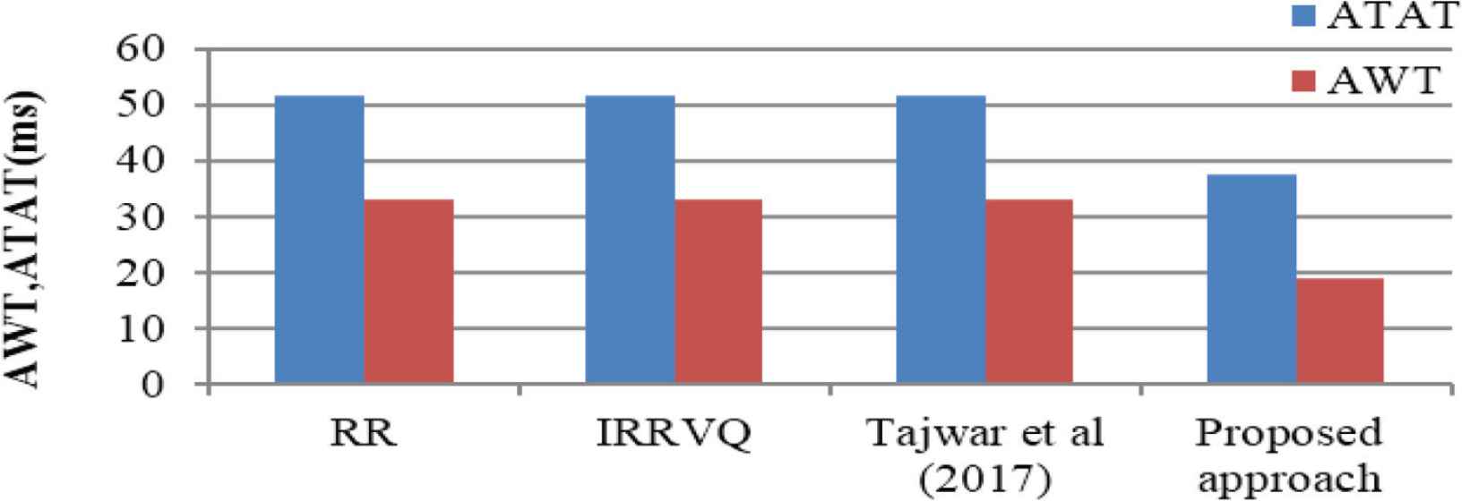
Comparison of RR, IRRVQ, Tajwar et al. [4] and proposed approach by taking ATAT and AWT (Case 2).

4.3. Case 3: Variable Arrival Time

Five processes P1, P2, P3, P4 and P5 arriving at time 0, 10, 12, 21 and 26 respectively with burst time 20, 200, 150, 230 and 75.

Table 5 shows the arrival time and burst time of processes. The comparison result of RR, IRRVQ, Tajwar et al. [4] and our algorithm is shown in Table 6. Figure 11 shows a graphical comparison of RR, IRRVQ, Tajwar et al. [4] and proposed approach in terms of ATAT and AWT.

Process	Arrival time	Burst time
P1	0	20
P2	10	200
P3	12	150
P4	21	230
P5	26	75

Table 5

Processes with variable arrival time (Case 3)

Algorithm	Quantum time (TQ)	Waiting time of each process	Average waiting time (ms)	Average turnaround time (ms)
RR	20	P1 = 0, P2 = 415, P3 = 383, P4 = 424, P5 = 234	291.2	426.2
IRRVQ	20, 55, 75, 50, 30	P1 = 0, P2 = 385, P3 = 233, P4 = 424, P5 = 54	219.2	354.2
Tajwar et al. [4]	20, 143, 52, 15	P1 = 0, P2 = 398, P3 = 123, P4 = 424, P5 = 54	199.8	334.8
Proposed algorithm	10, 105, 175, 200, 30	P1 = 0, P2 = 235, P3 = 8, P4 = 424, P5 = 144	162.2	297.2

Table 6

Comparison results (Case 3)

Figure 11

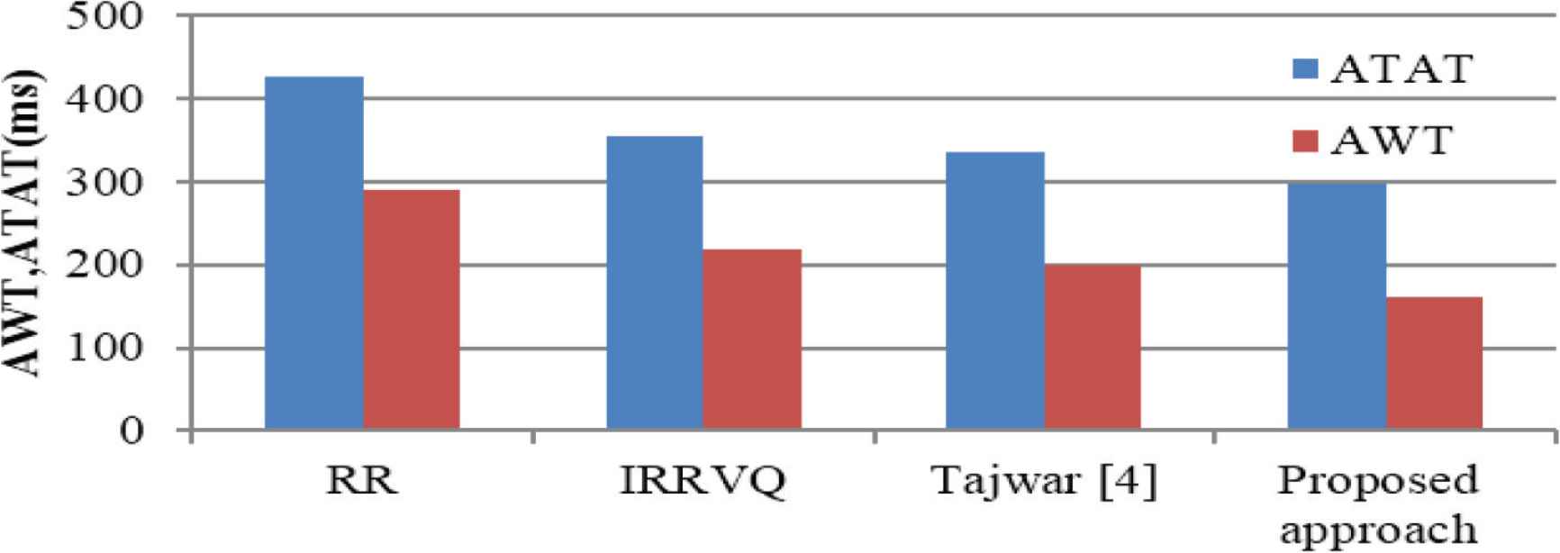
Comparison of RR, IRRVQ, Tajwar et al. [4] and proposed approach by taking ATAT and AWT (Case 3).

4.4. Case 4: Zero Arrival Time

The processes are arriving at time 0 with burst time 91.753, 263.115, 275.111, 280.222 and 352.609 respectively. The analytic model is applied to define the new order of tasks; in this case, the order will not change.

Table 7 shows the arrival time and burst time of processes. The comparison result of RR, AET-RR algorithm and the proposed algorithm is shown in Table 8. Figure 12 shows a graphical comparison of RR, AET-RR and proposed approach in terms of ATAT and AWT.

Process	Arrival time	Burst time
P1	0	91.753
P2	0	263.115
P3	0	275.111
P4	0	280.222
P5	0	352.609

Table 7

Processes with variable arrival time (Case 4)

Algorithm	Quantum time (TQ)	Waiting time of each process	Average waiting time (ms)	Average turnaround time (ms)
RR	25	P1 = 300, P2 = 941.753, P3 = 1004.868, P4 = 1000.09, P5 = 1005.312	850.404	1102.966
AET-RR	279, 274, 249, 73, 64, 25	P1 = 0, P2 = 963.753, P3 = 850, P4 = 876.111, P5 = 910.201	714.613	967.175
Proposed algorithm	263.115, 11.996, 316.4155, 36.1935	P1 = 0, P2 = 91.753, P3 = 354.868, P4 = 629.979, P5 = 910.201	397.3602	523.9264

Table 8

Comparison results (Case 4)

Figure 12

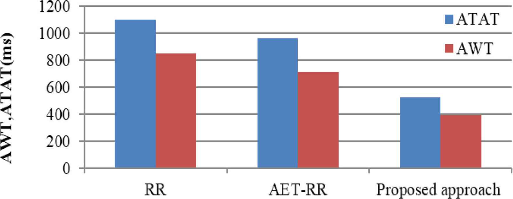
Comparison of RR, AET-RR and proposed approach by taking ATAT and AWT (Case 4).

4.5. Case 5: Variable Arrival Time

Five processes P1, P2, P3, P4 and P5 arriving at time 0, 15, 25, 35 and 40 respectively with burst time 597.801, 648.670, 649.659, 798.514, 827.617.

Table 9 shows the arrival time and burst time of processes. The comparison result of RR, AET-RR algorithm and the proposed algorithm is shown in Table 10. Figure 13 shows a graphical comparison of RR, AET-RR and proposed approach in terms of ATAT and AWT. In this section, five scenarios are used to show the effectiveness of the proposed approach compared to traditional RR, IRRVQ, Tajwar et al. [4] and AET-RR algorithms. The results obtained show a significant improvement with regard to the reduction of average execution time AWT and ATAT.

Process	Arrival time	Burst time
P1	0	597.801
P2	15	648.670
P3	25	649.659
P4	35	798.514
P5	40	827.617

Table 9

Processes with variable arrival time (Case 5)

Algorithm	Quantum time (TQ)	Waiting time of each process	Average waiting time (ms)	Average turnaround time (ms)
RR	25	P1 = 2030, P2 = 2287.801, P3 = 2931.13, P4 = 3274.644, P5 = 3347.261	2319.009	3023.461
AET-RR	597.801, 781, 746, 603, 383, 176, 125, 74, 25, 25	P1 = 0, P2 = 582.801, P3 = 2920.495, P4 = 2329.823, P5 = 2654.668	1697.557	2402.009
Proposed algorithm	298.9005, 648.670, 0.989, 813.0655, 14.5515	P1 = 0, P2 = 582.801, P3 = 1221.471, P4 = 1861.13, P5 = 2654.644	1264.0092	1968.4614

Table 10

Comparison results (Case 5)

Figure 13

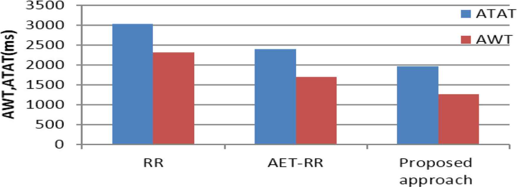
Comparison of RR, AET-RR and proposed approach by taking ATAT and AWT (Case 5).

5. CONCLUSION

There are several scheduling algorithms such as FCFS, Min–Min, Max–Min, SJF, shortest remaining processing time (SRPT), RR etc. These algorithms have several drawbacks: the task waiting for another task to complete its execution, the non-use of multiple parameters in the scheduling process, the ignorance of the type of task (heavy or light), and the use of a static time quantum etc.

In this paper, we aimed to overcome these drawbacks by proposing an improved Round Robin scheduling algorithm using a variable time quantum based on an analytic model. The proposed multiparameter analytic model calculates the cost of each task. The ready tasks list is sorted according to this cost. The proposed approach uses an optimal time quantum during the execution process based on the burst time of the processes existing in the ready list.

The results show that the proposed approach gives better performance than traditional RR, IRRVQ, Tajwar et al. [4] and AET-RR algorithms by reducing the waiting time and TAT which help in improving the system performance. In future works, the proposed algorithm will be improved to support and share multiple resources between tasks.

ACKNOWLEDGMENTS

This research was supported by the Algerian Ministry of Higher Education and Scientific Research, General Direction of Scientific Research and Technological Development.