
Customer Prediction using Parking Logs with Recurrent Neural Networks
Jeju National University, Jeju Island, South Korea. ycb@jejunu.ac.kr & mudassar192@hotmail.com
- DOI
- 10.2991/ijndc.2018.6.3.2How to use a DOI?
- Keywords
- Neural Network; Convolutional; Recurrent; Prediction; Traffic Patterns; Long Short-Term Memory; Vanilla
- Abstract
Neural Networks have been performing state of the art for almost a decade now; when it comes to classification and prediction domains. Within last few years, neural networks have been improved tremendously and their performance is even better than humans in some domains, e.g. AlphaGo vs Lee Sedol and Image Net Challenge-2009. It’s a beneficial factor for any parking lot to know that what would be a parking position at any given point in time. If we are able to know in advance that are we going to get parking tomorrow afternoon in a busy super store parking lot, its very beneficial to plan accordingly. In this paper, we predict customer influx in a specific departmental store by analyzing the data of its parking lot. We use this parking data to predict the customer influx and outflux for that parking lot as this parking influx is directly proportional to the customer influx in the store. We use Recurrent Neural Network on the top of two years of historical data. We generate promising results using this dataset by predicting the traffic flow for each hour for next 7 days. We further improve our performance on this dataset by incorporating three more environmental factors along with the parking logs.
- Copyright
- © 2018, the Authors. Published by Atlantis Press.
- Open Access
- This is an open access article under the CC BY-NC license (http://creativecommons.org/licences/by-nc/4.0/).
1. Introduction
Finding a sufficient parking space is a top priority during peak hours, especially during holidays. Parking is a major problem with cities, especially ones with a high population density. According to Donald C. Shop1, 34 percent of cars in a crowded area will travel in search of parking spaces during peak hours.it is difficult to find a place to park the car in big cities like Paris, Tokyo, Singapore or Seoul, especially if you have decided to leave during rush / office hours2. According to Caicedo and Robost3, drivers who know their surrounding areas; usually receive 45% success in finding parking places more than those who do not have general knowledge of the site. Consider Hangzhou(China) for example. As of 2017, there were 2.38 million vehicles on the roads but only 1.2 million parking slots available throughout the city4. If you decide to go to a supermarket, parking places around are at maximum capacity most of the time, leading to long queues and waiting times. It doesnot take long before customers start opting for another grocery store(due to these queues). For business owners, due to the limited number of parking spaces, customer flow will remain at constant maximum during the peak hours. However, when the peak hour expires, the parking space will be mostly vacant.
Many scientists have tried to solve this problem in several ways. This is a problem of allocating credits with weighted predictions for engineers and mathematicians. It about setting up initial weights using the right scales for various factors in the scenario to get the desired result. This problem of appointing credits is primitive one for them. Machine learning through neural networks is basically the application of this allocation problem only on a wider scale and at different levels. In deep learning, we learn these weights in many different layers to tailor output to the desired results.
Since the early sixties and seventies, there was a sufficient trend of Gradient Decent with Back Propagation (which is commonly used in the NN method today), but integration into the neural network began in the 1980’s. Due to its limitations on the architecture and performance of computer processing, focus on machine learning at the end of 80’s and 90s fell. Machine Learning got back onto main screen when it won visual recognition challenge in 2009.This success was due to major enhancements in terms of computer processing power which allowed multi-layer architectures in machine learning. Since then, machine learning has become commonplace in most areas. It has turned out to be a state of the art in the field of visual recognition and pattern recognition among many others.
Machine learning or deep learning uses two different types as its basic architecture. First type is known as Convolutional Neural Network or simply CNN. These networks are well suited for most scenarios of identifying images where data is independent of any time or on-demand restrictions. But for scenarios in which constraints of time or interdependency within data is observed, such as video or audio recordings or text, CNN will fail to pick up these dependencies. This problem can be solved by using a Recurrent Neural Network (RNN) which is the second type of neural network, and is well versed in time or data interdependencies. In very simple terms, it contains a memory component that allows it to store selective knowledge of the time line dependencies as opposed to CNN which doesn’t contain any memory component5.
Both CNN and RNN are subtypes of artificial neural network (ANN) or neural network (NN) simply. Typically, NNs contain 3 different types of layers. The first one is input layer from which input data is provided to the neural network. Then NN contains the hidden X layers. These hidden layers are abstraction layers; each of which depends on the abstraction submitted to it from its previous layer except for first hidden layer which works on data input layer. Depending on the complexity of the problem, this X can vary from 1 to several thousand. These hidden layers learn abstract concepts by learning the weight matrix of the input data. The last element in the NN structure is the output layer, which may contain 1 to more neurons. It can generate two different kinds of outputs. It can be numeric values (the case of prediction or RNN) or category (in case of Classification or CNN).
Every layer in any neural network are composed of neurons. Neurons usually work in a very simple way as they get all the input attached to it via input lanes, multiply them it with the weight matrix, and then apply the function to generate its output. This function can range from simple aggregation of inputs to complex nonlinear functions. A simple neuron works on basis of the following equation.
- x0 =
Initial bais (usually defaults to 1).
- x1..xn =
inputs to neuron.
- w1..wn =
weights associated to each input.
Consider the scenario of a grocery store manager. If he can have prior information about the customers influx then he can take many fruitful decisions on its basis. If the forecast of customers for next day is low then he can employ less salesman for tomorrow. Similarly if forecast is high then he can have extra salesman for that day. He can also plan other utilities (e.g. electricity, Gas) saving him some more resources.
In this paper; we predict customer Influx for a specific departmental store using its parking logs. We use data spanning two years as input for our scenario. We predict the number of cars that will be visiting the departmental store for each hour in next 7 days. We use Recurrent Neural Network to perform this prediction. We also use variations in architecture as well as different types of cells within RNN.
Rest of the paper is divided into 5 sections. Section 1 was introduction, section 2 is related work, section 3 is data analysis, section 4 is proposed methodology and 5 includes conclusion.
2. Related Works
The problem we are working on is customer prediction using parking data. To the best of my knowledge there is not much work in parking predictions using machine learning directly. The next most important and relevant area is the traffic forecasting. Manoel, Castro-Neto and Young-Seon Jeong6 used supervised learning to predict short-term traffic. They utilized support vector machine and statistical regression (OL-SVR) to predict traffic under normal and unconventional conditions. In addition, they used PeSMS data and compared its results to the maximum GOS possibilities and achieved the same or better performance under common conditions. Richer and Martino7 worked on a different approach to predict parking intensity in a specific area. They considered the factors that cars dont have strong telemetric systems and ones that are installed have serious storage capacity issues. They created a model and pushed it into the vechicle’s navigation system. Their proposed model wass trained over historical data of past 5 months and their solution required 99% less space and was around 70% percent accurate. The problem with this approach was that it guided the users towards free parking based on historical data of the place for last 5 months and once model was pushed into navigation system it can only be replaced by newer version. They investigated the tradeoff between accuracy vs graunality and 70% was their best accuracy.
Reinstadler and Ricci8 have proposed time series forecasting on parking data for 2 parking lots in bolzano. They used an opensource data mining tool WEKA that uses combination of machine learning and data mining techniques to analyize data. Authors created two different subsystems where tf-model was responsible for generating the forcasts for parking in xml formatting and second component tf-forecast was responsible for broadcasting it to internet. In their work, two different parking lots were used as data source; Parking 108 with 992 parking spaces and parking 116 with 770 parking spaces. They produced varying results with different configurations in their work. In general they did not specify any numeric error value in terms of RSME or any other metric. Tooraj and Petros9 have used parking data to propose a multivariate autoregressive model that considers both temporal and spatial correlations which account for parking availability. Their proposed model recommended users to choose parking where there is highest probability of finding at-least one parking spot. The basic difference of this approach is that it has statistical basis and machine learning is now proven to provide better results then traditional statistical methods.
Yu and Wo10 used RNN’s Spaciotemporal abilities and LSTM to predict traffic. They converted traffic features into images and then trained RNNs on those images to predict traffic flow. There was no comparison with related methods in their work. Sherif Isaac11 proposed to improve traffic prediction using four different architectures. His work compared neural networks with LSTM, the co-adaptive neuro-fuzzy inference system (CANFIS) and typical modular networks. He utilized different video lengths in range of 1 to 10 minutes. Author concluded that no single algorithm works best for all conditions because different algorithms perform better under different conditions. Rose Yu, Stephan Zheng12 utilized the RNN-trained cellar for the long-term prediction traffic. The Higher Order Generalization were used above RNN to capture long-term temporal dependencies. Their RNN was good in both linear and nonlinear environments. Their work displayed better performance than both LSTM and Vanilla RNN on their dataset.
These works are mainly concentrated on road traffic and are fruitful from the perspective of traffic density and patterns on the road. In the scenarios we analyze, these are different usage scenarios, as we are considering data for specific parking conditions, which may be a superstore or a big mart, focusing on its customer patterns and uses. The importance of these works is that they use the same neural network we use at work to handle traffic density, but we focus on parking. We focus on fixed parking and forecast customer traffic related to our customers. This makes the problem different from the above works in terms of goals and implementation.
There are very few works on machine learning in terms of customer prediction using parking information. In the proposed work of Philip and Thompson13, they predicted the churn rate for customers. Their focus was not on any company specific data but on independent customer characteristics (which are generic for all customers). Like Philip and Thomoson; most of the commercial companies focus on using their available customer data to predict customers; which only contain customer statistics and no indication of parking capacity and availability. The sample data set includes the customer’s personal information such as name, gender, age, credit score, etc.
In terms of parking forecasting, there is not much work to predict parking spaces. Fabian and Sergio14 summarized different ways of extracting parking data from different inspection vehicles. Authors collected data from different inspection vehicles and applied machine learning to determine the legitimacy and availability of these parking spaces. They used taxi’s sensors and GPS within it. In their work; they utilized different virtual sensors installed in taxis to collect parking data They map the data to a map with the help of GPS. Using these data and maps, they applied random forest classification to predict empty parking spaces.
Zheng, Rajasegarar and Leckie15 tried to predict the occupancy of parking lots at any given date and time in their work. They have proposed three different feature sets and studied their performance. These features include probable occupancy time, time steps to be predicted and their combination. Authors also utilized multiple prediction techniques and compared their results. These include Regression Tree, Support Vector Regression (SVR), Neural Networks applied on San Francisco Parking Dataset of almost 1 month (12th Aug 2013 to 22nd Sep 2013) and on Melborne dataset for 1 year (1st Oct 2011 to 30th Sep 2012. They concluded that regression tree outperforms both SVR and NN in terms of performance using historical occupancy rates and datetime.
Xiao Chen16 tried to predict parking space in San Francisco area. They utilized SFPARK data for 6 months (1st July 2013 to 29th December 2013). The data includes latitude, longitude, place name , lot capacity, captured slots as well. They work on ARIMA , SVR, Linear Regression, and Feed Forward Neural Networks. They conclude that that ARIMA has most error with 8.09% while NN perform best using logestic regression with 3.57% error. Although the work is relevant but its very less in terms of content.
Vlahogianni and Kepaptsolglou17 use onsite sensors and parking data on the street to predict the availability of short and nearby rental parking spaces. They utilized data used for 5 minutes from the first hour to predict the occupancy of rest of the hour. Eran and Christopher18 used predictive parking rates, past occupancy rates and location features to predict the price of a parking space. They also studied its impact on the surrounding parking spaces and proposed a price that would make the surrounding area more profitable.
In our proposed work, we predict customers intake in specific store by predicting traffic within its parking lot based on its parking data. This is a relatively new spectrum and not much work has been done to predict customer behavior using traffic data.
3. Data Analysis
In this project, the data received was based on 2013 January till December 2014. We started to analyze this data and discovered some patterns from this data. The raw data was formatted in 4 columns. First column was cars license plate number. The number was in format 00-LL-0000, where 0 denotes for numbers and L for single Korean alphabet. There were some exception to this format but number was quite small (0.01% of dataset). Next column was the incoming time that was followed by the outgoing time. Both these times were formatted in format YY-MM-DD HH:MM. Last column was of the discount type. This column referred to the discount given to the car when it exited from parking lot. These discounts were given to senior citizens, low pollution cars (usually electric), or to a disabled person as shown in figure 2.
This column also included some garbage values which were not falling into any category. These values were discarded and default value of ”Normal” was used instead while cleansing data.
During our initial analysis we found this data to contain multiple patterns. To be precise 3 major patterns were generated by the data. First was that there was high intake of cars during the morning hours of the day while in the late hours most of the load was on out gate. Preferred pattern was that cars started to come right after 8 AM but usually relatively large number of cars came around 10 AM onwards. Most of the cars left after some reasonable time (usually within half an hour) but some cars stayed till back-end of the day. In evening hours there was predictively more load on the outgoing gate. Figure 1 shows the following pattern for multiple days of week generated from the raw data.

Parking traffic trends for Monday, Saturday, Sunday and Overall (hour-wise)
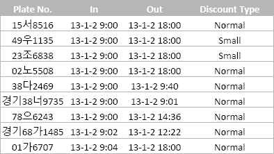
Raw Parking Logs: Sample Input
Second important pattern was that we saw reletavly less cars in parking in first week of the month. For the second, third, and last week, number of cars were somewhat same (although still more then first week). This was a surprise for us as we were expecting an inverted result. The result for whole month averaged over 2 years of data is shown in figure 3
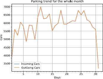
Trend for complete month
Third and final pattern was that people preferred to come on monday as usually there were more cars utilizing parking facility on Monday then rest of the weekdays. Monday usually had the most traffic with a gradual decline on Tuesdays, wednesdays and Thursdays. Friday again had more traffic as people tried to finish grocery before weekend starts. On Saturday, the customers come in early hours but in less numbers as compared to other weekdays and that too in early hours of the day. On Sundays, parking was closed therefore parking lot was empty. Another slight trend was that there was a spike in traffic after some public holiday as well.
A good example was that after chousak holidays there is a monday like spike on weekday even though its not monday. Figure 1 shows the behavior of cars on Mondays, Saturdays, Sundays and Overall (averaged over all the days of the week for two years).
4. Proposed Methodology
After the initial analysis, we converted this dataset into Day based grain. The initial format that data was converted was that it had 4 different fields. First was date, followed by the cars that came into the parking lot. Then the cars that exited the parking on that day and the last field was number of cars parked overnight. It converted the 177,000 logs spanning over two years into 729 days as shown in figure 4.
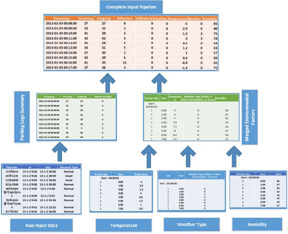
Data merging for the input of Recurrent Neural Network
We then did feature scaling on this dataset. Reason for the feature scaling is that it helps the neural network to converge more quickly. The logic behind this phenomenon is the fact that usually when we are using multiple features, then they may be of different scales. A simple example in this regard was that the incoming and outgoing cars were varying between scales of 300–700 but the cars parked overnight never exceeded single digit (0 - 9). Application of feature scaling will also become more evident as we will further go down in paper (when adding more features). For feature normalization we used following formula.
Where e : Eulers Constant; Added to remove division by zero possibility.
We divided this dataset into two portions for our machine learning process. Seventy percent of this dataset was separated for training and rest of thirty percent for testing. All this data is summarized in table 1. In machine learning, there are two basic kinds of neural networks. First are convolutional neural networks. These networks are usually utilized when we are categorizing some sort of data. One of the best examples would be image classification, where CNNs are now state of the art phenomenon with results even better then human benchmark. These networks work very well for classification and on those datasets where there is no relation between the flow of input data. In other words, CNN does not consider that all the data required to classify an image or to do a task is in the input provided. For our scenario we have time factor and consecutive examples have impact on successive one within dataset. This is accounted by the other major kind of neural network, i.e. recurrent neural network.
| Feature | Value |
|---|---|
| Basic Data Input Type | Car Entry Logs |
| Data Format | Plate Number, Incoming Time, Outgoing Time, Discount Type. |
| Logs Start Date | 1st Jan 2013 |
| Logs End Date | 31st Dec 2014 |
| Total Records | 177000 Entries |
| Records Span | 2 Years (729 Days) |
| Aggregation Level | Days |
| Train Data | 70 % |
| Test Data | 30 % |
| Normalization Formula | (Feature - Min) / (Max - Min + e). |
Parking logs summary
This network works best with the data that has the time factor dependencies. In other words, whenever we have data where some event in time has an impact over some other event happening later in time then RNN performs best. We experimented with two different categories of Recurrent Neural Network. First Vanilla RNN which utilizes standard memory cell and only gives priority to the most recent information. LSTM (Long Short-Term Memory) differs from vanilla RNN in this context. Its Memory component is more sophisticated and LSTM intelligently decides which information to store. Complete picture of our system architecture is shown in figure 5.
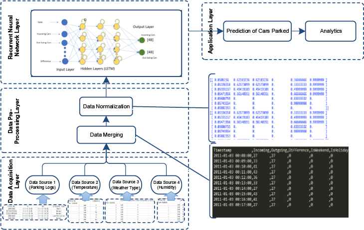
System architecture
Initially, we used seven days of data as an input and predicted two different values for each of next seven days. First was the number of cars that came into the parking and second was the number of cars that left the parking on that specific days. We took multiple combinations of hidden layers ranging from three till fourteen. The metric we used for accuracy was RMSE (Root Mean Square Error). All this information is summarized in table 2.
| Parameter | Value |
|---|---|
| RNN Type | Vanilla, LSTM |
| Input Layer | 1 * [7 days * 24 * 9 features] = 1512 Neurons |
| Output Layer | 7 * 2 * 24= 336 Neurons |
| Hidden Layers | [3, 5, 7, 10, 12, 14] Layers |
| Learning Rate | 0.1 , 0.01 , 0.001 , 0.005 ,0.0001 , 0.00001 |
| Sequence Length | 7 Days (7 * 24 * 9 = 1512) |
| Iterations | 1,000 , 2,000 , 10,000 , 20,000 |
Recurrent Neural Network Configurations
Our initial results were not that good. We were not getting RSME below 0.30. A further investigation led us to conclusion that we were missing the weekend and holiday patterns, and most of the error was due to miscalculation on Saturdays, Sundays, and on public holidays. This led us to incorporating two additional features into our preprocessed dataset.
We added a feature for weekday which had values from 0 (Monday) to 6 (Sunday) and a boolean feature isHoliday which was set for public holidays as 1. After adding these features our network started to depict much better results. Our RSME was dropped from 0.30 to 0.19 in case of RSME and 0.23 in case of vanilla RNNs.
We decided to integrate a set of new features and reduce the predicting grain as well. We worked on original parking data and converted it into hour-based summary instead of day-based summary. The reason for this is explained in Conclusions section. Secondly, we gathered environmental data for this time period and integrated that with our hour-based parking logs as well. We considered three different features to be added. First was weather type. It had 4 different values (sunny, rainy, snowy and cloudy). Next feature was temperature on that specific hour and last feature was humidity. Adding these features takes number of features to 9 as summarized in table 3.
| Feature | Value |
|---|---|
| Basic Data Input Type | Processed Logs |
| Data Format | Hour, Incoming Cars, Outgoing Cars, Already Parked Cars, isHoliday, Weekday, Temperature, Humidity, Weather Type |
| Logs Start Date | 1st Jan 2013 |
| Logs End Date | 31st Dec 2014 |
| Total Records | 177000 Entries |
| Records Span | 2 Years (729 Days) * 24 hrs [17486 entries] |
| Aggregation Level | Days |
| Train Data | 70 % |
| Test Data | 30 % |
| Normalization Formula | (Feature - Min) / (Max - Min + e). |
Preprocessed dataset summary
After changing the dataset, we trained our recurrent neural network on this dataset. The input layer contained 7 (Days) * 24 (Hours) * 9 (Features) = 1512 neurons. The output layer contained 7(days) * 24 (hours) * 2(features) = 336 neurons. Hidden layers were experimented with were again 3 to 14. Learning rates varied from 0.00001 to 0.1. We tested them on both Vanilla and LSTM RNNs.
Results were much better than original 6 features. We were able to achieve RSME of 0.11906 with LSTM and 0.14580 with Vanilla RNN. We experimented with different configurations of epochs but it seems that 20,000 is the magic number. Before 20,000 there is underfitting and if epochs are increased then overfitting starts to show up. We found optimal layers to be 7, optimal structure to be RSME in RNN and optimal learning rate to be 0.14580.These results are summarized in table 4.
| Configurations | Vanilla RNN | LSTM |
|---|---|---|
| Iterations | 20,000 | 20,000 |
| Learning Rate (Optimal) | 0.00001 | 0.01 |
| Memory | Standard | LSTM |
| Optimal Number Layers | 7 | 7 |
| RSME(Optimal) | 0.14580 | 0.11906 |
Experimental results using vanilla RNN and LSTMs
5. Conclusion
In this paper, we proposed a noval approach to calculate customers influx for a specific departmental store using its parking logs. We predicted the influx and outflux in its parking logs and using that we can safely predict that inflow of departmental store would be directly proposional to this rate. We had 2 years worth of parking logs on top of which we applied recurrent neural network after some preprocessing and cleansing. We were able to produce state of the art results in this regard achieving RSME of about .119 on this dataset. Results showed that LSTM perform better then vanilla in our scenario by about 0.03 (absolute) in terms of RSME. When only Parking Logs data was used as input to RNN; RSME was about 0.07(absolute) less then when using whole data(both parking logs and environmental data).
The reason for the improvement in results is two folds. One is adding environmental factors. Their impact is eminent as its very logical that if its snowing and temperature is down then the probability of having high amount of customers is very slim and similarly is the case of vice versa. These extra three features were helpful in improvement in performance but they do not fully justify the jump from 0.199 to 0.11. The more critical factor in this regard is the grain devolution. As we devolved the grain we got two benefits. First, RNN was able to capture the dependencies that existed within a day. For example, if someday there is high trend of incoming cars in earlier part of day, there is high probability that there would be high number of cars leaving in later part of that day. Another imminent factor is that reducing this grain size increases the training data size. Now each record is 24 records in new dataset and that means dataset is now increased 24 folds. This is the more critical factor in terms of improving this performance. The more data we had to train on, the better results were generated by the recurrent neural network on it.
6. Acknowledgement
This research was financially supported by the Ministry of SMEs and Startups(MSS), Korea, under the Regional Specialized Industry Development Program (Grant No. C0515862) supervised by the Korea Institute for Advancement of Technology (KIAT).
References
Cite this article
TY  - JOUR
AU  - Liaq Mudassar
AU  - Yung-Cheol Byun
PY  - 2018
DA  - 2018/07/31
TI  - Customer Prediction using Parking Logs with Recurrent Neural Networks
JO  - International Journal of Networked and Distributed Computing
SP  - 133
EP  - 142
VL  - 6
IS  - 3
SN  - 2211-7946
UR  - https://doi.org/10.2991/ijndc.2018.6.3.2
DO  - 10.2991/ijndc.2018.6.3.2
ID  - Mudassar2018
ER  -