
Exchange Rate Dynamics and Trade Balance in Selected African Countries
 , Abdulrasheed Isah2,
 - DOI
- 10.2991/jat.k.201218.001How to use a DOI?
- Keywords
- Trade balance; exchange rate; asymmetry; NARDL
- Abstract
African countries have over the years experienced persistent current account deficits. The role of asymmetries in explaining the response of trade balance to exchange rate movement has not received adequate attention as linear models dominate extant empirical literature. In this paper, we examined the impact of exchange rate on the trade balance in five African countries using both linear and nonlinear autoregressive distributed lag models to analyze data for the period 1980–2018. The linear model revealed that the J-curve holds in Uganda in the short run, whereas evidence of long-run J-curve effect was found only in Algeria. However, the nonlinear analysis showed that the short-run J-curve holds for South Africa and Uganda whereas a long-run J-curve effect was found in Algeria and Uganda. The results make a case for modeling asymmetries as the nonlinear model performed relatively better. An important policy implication is the need to address structural imbalances in the economy to leverage on the exchange rate and trade policies to improve trade outcomes.
- Copyright
- © 2020 African Export-Import Bank. Publishing services by Atlantis Press International B.V.
- Open Access
- This is an open access article distributed under the CC BY-NC 4.0 license (http://creativecommons.org/licenses/by-nc/4.0/).
1. INTRODUCTION
The link between exchange rate and trade balance has important implications for the formation of a regional trade agreement. The recently signed Africa Continental Free Trade Area (AfCFTA), which seeks to foster regional integration, easily comes to mind. The agreement entails the liberalization of trade barriers across Africa intending to achieve stronger intraregional trade, increased investment flows, and rapid growth. The deal is also expected to help buffer the region against adverse shocks and long-term deterioration in terms of trade, particularly with non-African trading partners (United Nations Economic Commission for Africa, 2020). However, limited export diversification has hindered the competitiveness of African countries, which are mostly resource-dependent, making them highly vulnerable to commodity shocks.
The need to monitor external imbalances is important in African countries, where the current account deficit has persistently widened. For instance, after decreasing to an estimated 4.6% of the Gross Domestic Product (GDP) in 2019, the median current account deficit in the region is projected at 5.8% of GDP in 2020, reflecting a deterioration in the current account balances of oil exporters because of the sharp fall in oil prices (World Bank, 2020a). The North African countries recorded an average deficit of 4.4% of GDP in 2019 and a projected deficit of 11.4% of GDP in 2020 (African Development Bank, 2020). This is largely driven by the 20% and 19.8% deficits recorded in Algeria and Libya, respectively. These developments suggest that knowledge of the extent and nature of the relationship between exchange rate and trade balance is very crucial to African policymakers particularly for designing and managing both exchange rate and trade policies to achieve desired macroeconomic outcomes.
Although the exchange rate is a veritable instrument to address trade deficits, African countries have not sufficiently harnessed the competitiveness gains of a devaluation (or real depreciation). For instance, while the central bank of South Africa announced it will not continue to intervene in the foreign exchange market, the Bank of Uganda announced that it stands ready to intervene in the foreign exchange market to smoothen volatility (World Bank, 2020a). In Nigeria, the exchange rate has been officially adjusted by 15% with ongoing efforts to unify the various segments of the exchange rate market. Apart from Egypt and Mauritania, North African countries still maintain foreign exchange controls as there exists a significant difference between the official and parallel rates in Algeria.
The relationship between real exchange rate and trade dynamics has received significant attention, especially within the context of the Marshall–Lerner condition, which posits that if the sum of import and export demand elasticities of a country exceeds unity, a real depreciation would have a favorable effect on the trade balance. However, Bahmani-Oskooee (1985) notes that a country can fulfill the Marshall–Lerner condition but still experience a deterioration of the trade balance. For instance, a real depreciation can lead to a fall in exports because the export-oriented sectors require imported intermediate and capital goods. This lends support to the growing concern that trade liberalization should be accompanied by reforms and adjustments that address productivity constraints. This is because export expansion can be negatively affected by currency depreciation or, even worse, trigger a balance of payment crisis (Arize et al., 2017).
An understanding of the J-curve can help countries prepare for market expansion and promote more coordinated exchange rate and trade policies. As African countries relax trade restrictions, sound exchange rate management will be essential for maximizing the gains from intraregional trade flows and industrialization (United Nations Economic Commission for Africa, 2020). Similarly, knowledge of how the trade balance in African countries is influenced by changes in the real exchange rates can help policymakers during trade negotiations with trading partners, thereby helping to achieve better trade deals. Nusair (2016) notes that the nexus between trade balance and the exchange rate is of paramount importance to policymakers because it provides insights toward regional trade policy formulation and implementation.
An important gap in extant studies is the assumption of symmetry in the dynamics of the exchange rate, and this largely conforms with empirical regularity for most African economies where a real depreciation (or devaluation) is rife compared to a real appreciation. However, Bahmani-Oskooee and Fariditavana (2016) have argued that exchange-rate changes could have asymmetric effects on the trade balance. Similar evidence has been documented by Bahmani-Oskooee and Mitra (2009) for India, Nusair (2016) for European transition economies, and Bahmani-Oskooee et al. (2017) for Bangladesh. These findings underscore the need to account for asymmetry.
Economic theory suggests that a depreciation makes exports less expensive, leading to a gain for exporters as demand increases. By contrast, a real appreciation of the domestic currency makes exports more expensive and less competitive in terms of foreign currency. The demand for domestic exports falls if the domestic price does not contract. Yet if the real appreciation is significantly high, lowering export prices becomes difficult because it could substantially reduce the profit margins of domestic exporting firms. This is because export prices are often sticky downward in response to a real appreciation compared with a depreciation (Nusair, 2016).
The main motivation of this paper is that evidence on the J-curve hypothesis can provide valuable inputs for trade and exchange rate policies used by governments to correct external imbalances and mitigate the impact of shocks. Specifically, we subject the J-curve to empirical scrutiny through the lens of asymmetric effects of real depreciation and appreciation, which have not received adequate attention. Moreover, the use of both linear and nonlinear Autoregressive Distributed Lag (ARDL) models would shed more light on the J-curve phenomena in African countries. Thus, the main objective of this paper is to investigate whether the J-curve hypothesis holds in five African countries: Algeria, Cameroon, Nigeria, South Africa, and Uganda. These countries are selected not only because the data is available, but most importantly because they serve as key case studies from all the subregions of Africa. Moreover, the selected countries individually account for a significant share of GDP in their respective subregions. Consequently, a trade shock in these countries could spill over to other economies within the subregion. We also expect that an exchange rate shock could adversely affect intraregional trade flows, and more especially the external balance of the relatively smaller countries in the subregions that the selected countries represent.
The rest of this paper is structured as follows: Section 2 provides a background of the paper whereas Section 3 reviews related literature. Section 4 describes the underlying theory and methodology. Section 5 discusses the findings and Section 6 concludes.
2. TRADE AND EXCHANGE RATE DEVELOPMENTS IN AFRICA
In recent decades, trade between African countries and the rest of the world has significantly increased as a result of globalization. Although the degree of trade openness varies across the continent, African countries are generally open economies with significant links to other regions and countries through finance and investment channels as well. According to Moussa (2016), for the periods 1981–1990 and 2000–2014, average trade openness of sub-Saharan African countries rose from 37% to more than 65%. This positive trend could be explained by the reduction of trade and investment given the plethora of agreements pursued at the bilateral and multilateral levels. The spread of information and communication technologies, the rise of global value chains, as well as the growing importance of developing countries in global trade, have also contributed (World Bank, 2020). Trade can generate foreign exchange necessary to finance imports of intermediate goods for domestic industries, with positive implications for job creation, poverty alleviation, and growth in African countries.
However, the increased participation of many African countries in global trade has been associated with substantial widening of the trade and current deficits in recent years (Figures 1 and 2). The current account balance was about $1.1 trillion in 2018, down from $1.5 trillion in 2017, whereas the current account balance as a share of GDP increased from 5.8% in 2017 to 6.2% in 2018. The high deficit experienced in current account is more pronounced in resource-dependent economies such as Nigeria and Algeria, which are prone to volatile global commodity market conditions. Meanwhile, the importation of intermediate and high value-added goods has increased substantially across Africa, thereby contributing to unfavorable trade balance for many African countries during the same period. Similarly, Cameroon, Uganda, and South Africa have been recording current account deficits consistently over the past 20 years. However, it should be noted that sub-Saharan African countries experienced intermittent trade surpluses, specifically during 1985–1990 and 2000–2008. Moussa (2016) notes that the surpluses were attributed to the decrease in domestic demand and lower imports in the contexts of Structural Adjustment Policies of the 1980s, as well as high commodity prices during the early 2000s until the financial crisis of 2007–2009. Yet, although the region recorded a trade surplus between 2000 and 2008, only eight out of 45 economies had a trade surplus and only eight experienced current account surpluses. Meanwhile, about 33 countries had trade deficits within the period. Persistent trade deficits in African countries indicate a deep lack of competitiveness of local firms relative to foreign competitors, which exacerbate import dependence.
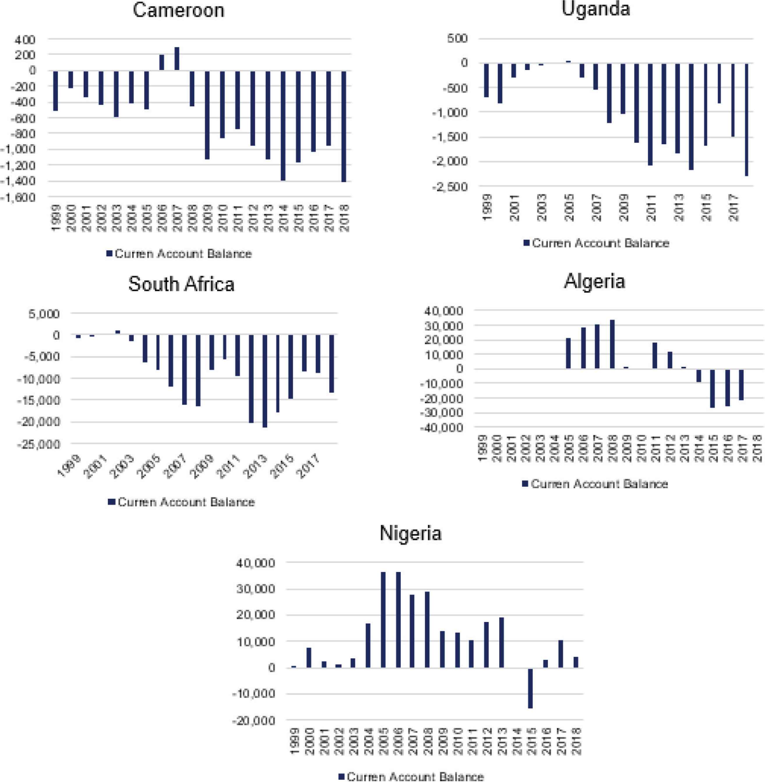
Current account balances in selected African countries (US$ million). Source: IMF International Financial Statistics, 2020.
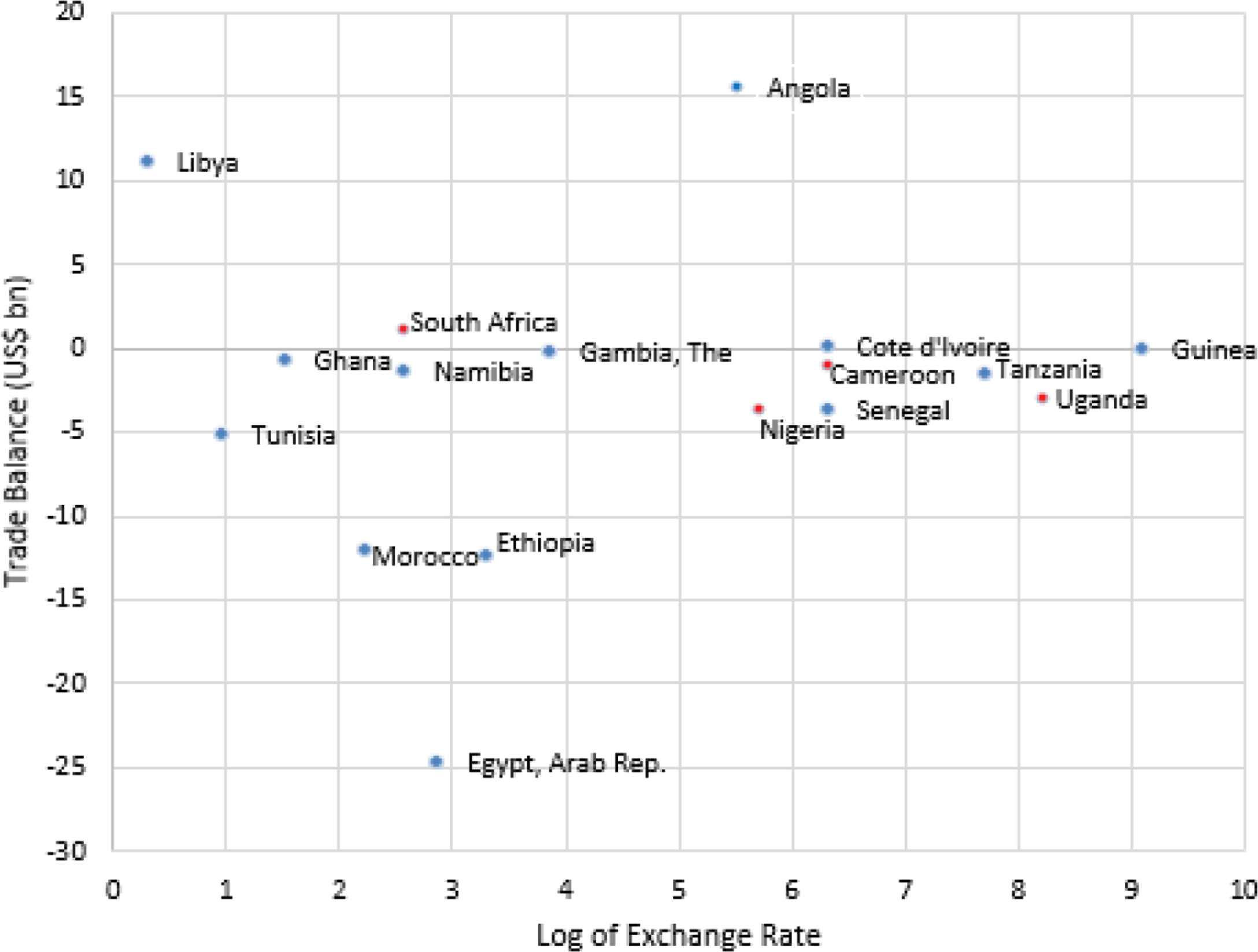
Trade balance and exchange rate in Africa. Source: World Bank, World Development Indicators, 2020.
There is a significant exchange rate variation among African countries (Figure 2). This could be partly explained by the different exchange rate regimes and the structure of the external sector. For instance, Nigeria is highly dependent on crude oil exports, and thus its current account balance is positive. The official exchange rate has been adjusted by 15%, with ongoing efforts toward the unification of the various exchange rate windows. In Angola, the central bank allows for a flexible exchange rate regime, whereas Botswana maintains a crawling peg. The central bank in South Africa announced it will continue its longstanding practice of not intervening in the foreign exchange market. The combination of the high exchange rate and negative trade balance has magnified external sector vulnerabilities. Figure 3 shows that South Africa and Ghana have the lowest exchange rate whereas Uganda and Cameroon have the highest domestic currency price. Amidst the shortage of scarce foreign exchange inflows, the Bank of Uganda remains committed to intervening in the foreign exchange market to smoothen excess volatility.
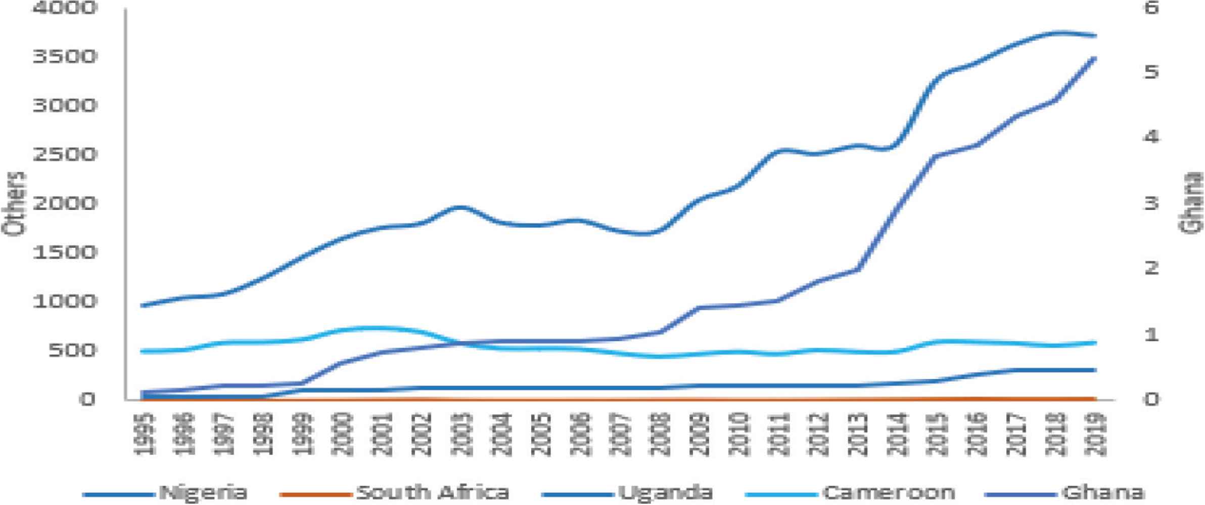
Exchange rate movement in selected African countries (local currency per US$). Source: World Bank, World Development Indicators, 2020.
3. LITERATURE REVIEW
3.1. Theoretical Background
The J-curve can be traced to the theoretical exploits of Magee (1973). The model assumes that an improvement in a country’s trade balance does not instantaneously translate to an appreciation of the domestic currency. This is because there may be outstanding contractual obligations that need to be enforced. This suggests that there is a time lag during which consumers and producers adjust to exchange rate changes. The absorption and elasticity approaches to balance of payment have dominated the analysis of exchange rate and trade. These models seek to ascertain whether a devaluation (or depreciation) of the exchange rate leads to a current account deficit. Whereas the elasticity approach focuses on price effects, the absorption approach is concerned with income effects. Ample evidence suggests that the two are not mutually exclusive but rather complementary (Krugman et al., 2018).
The elasticity approach, also referred to as Marshall–Lerner condition, states that in all other things, a real depreciation will improve the current account of a country if the volumes of exports and imports are sufficiently elastic to the exchange rate (Krugman et al., 2018). The model assumes that a devaluation can have a volume and/or price effect such that the former could reduce the trade deficit whereas the other could exacerbate it.1 Thus, the net effect is based on whether the price or income effect is larger following an exchange rate devaluation.
The absorption approach, by contrast, seeks to explain the impact of changes in exports and imports on the trade balance via income effects (Pilbeam, 2006). The current account imbalance is the difference between domestic output and spending. Thus, increasing domestic income relative to absorption could help address current account deficits (ibid.). Both the elasticity and income approaches are complementary. For instance, it is expected that income will increase if exports exceed imports provided the Marshall–Lerner condition holds. However, if the condition does not hold, exports rise by less than imports thereby reducing income. If income effects are considered, the elasticity condition of a positive effect of depreciation on trade balance will be affected.
Pilbeam (2006) broadly categorized economists into two: (1) elasticity optimists, who argue that the sum of the elasticities is greater than 1, and (2) elasticity pessimists, who contend that the sum of elasticities is less than unity. This means that the overall trade effect of a devaluation is context-specific. Further theoretical developments incorporate dynamics in the Marshall–Lerner condition. This is because the sum of the price elasticities might be lower in the short run compared with the long run, and the condition may not hold immediately, thereby exhibiting a J-curve pattern. Krugman et al. (2018) note that the sum of the elasticities is less than unity for most countries, and this prompts an immediate deterioration of the current account following a devaluation.
3.2. Empirical Literature
Several empirical studies have examined the long- and short-run relationships between the trade balance and exchange rate using different samples, datasets, models, and estimation procedures. Yet, the empirical evidence on the J-curve remains inconclusive.
A sizable body of the literature indicates the existence of the J-curve. For instance, Bahmani-Oskooee (1985) found that the trade balance of South Korea, Greece, and India significantly improved in the long run after a brief deterioration following a devaluation. However, the evidence for Thailand indicates that trade balance improves for five quarters after devaluation but deteriorates thereafter. Using vector error correction and Granger causality techniques, Akonji et al. (2013) found evidence of the J-curve in Nigeria whereas Hussain and Haque (2014) found evidence in support of the J-curve hypothesis in a sample of 49 African countries for the period 2000–2010 based on dynamic panel data approach.
Another strand of the literature does not confirm the existence of the J-curve phenomenon. For instance, Ziramba and Chifamba (2014) found that the real effective exchange rate has a negative long-run impact on the trade balance, suggesting that the J-curve does not hold in South Africa for the period 1975–2011. Similarly, Adeniyi et al. (2011) found that the J-curve holds only in the case of Nigeria, whereas an “inverted-j” was found in the case of Gambia and Ghana. They find no clear pattern of the J-curve in Sierra Leone. Moreover, Cergibozan and Ari (2017) found no evidence for the J-curve hypothesis in Turkey between 1987 and 2015.
Furthermore, the majority of the empirical literature presents conflicting results regarding the J-curve effects. For example, Bahmani-Oskooee and Ratha (2004) found no evidence of the J-curve in the short run but not in the long run based on a sample of the United States and its 18 trading partners over the period 1975–2000. The study also shows that the trade balance is affected by domestic and foreign income. Similarly, Hsing (2008) showed that the J-curve effect only existed in Chile, Ecuador, and Uruguay out of the seven Latin American countries considered. Bahmani-Oskooee and Gelan (2012) examined the existence of the J-curve in eight African countries (Burundi, Egypt, Kenya, Mauritius, Morocco, Nigeria, South Africa, and Tanzania) and found that the J-curve hypothesis does not hold in the short term in all of these countries. However, the long-run impact of a real depreciation was favorable only in Egypt, Nigeria, and South Africa. Bahmani-Oskooee and Mitra (2009) found no significant relationship between the real exchange rate and the bilateral trade balance between India and United States at the industry level as only eight out of 38 industries lend support to the existence of the J-curve. Specifically, although the real depreciation of the rupee has short-run impacts, these effects last into the long run in almost half of the industries considered.
More recent empirical works have begun to consider the potential asymmetry in the nexus between a real depreciation and appreciation and the trade balance. For instance, Bahmani-Oskooee and Baek (2019) assess the existence of the J-curve phenomenon between South Korea and its 14 trading partners using both the linear and nonlinear ARDL approaches. The authors found that the former lends support for the J-curve effect in seven countries, whereas the latter did not show any evidence of the J-curve effect in 10 countries. The findings also show that asymmetric effects were more pronounced in South Korea’s trade with Asian countries, suggesting that asymmetric effects may be trade partner-specific. Nusair (2016) found no evidence of the J-curve phenomenon in a sample of 16 European countries using a linear approach. However, the nonlinear model shows that the J-curve holds in 12 countries. In another study, Arize et al. (2017) found that when depreciation and appreciation are decomposed, the former has a significant effect on the trade balance, suggesting that asymmetries matter. Bahmani-Oskooee et al. (2017) investigated the J-curve phenomena between Bangladesh with 11 trading partners using linear and nonlinear approaches. The linear estimates showed that the J-curve holds in one country whereas the nonlinear variant indicates that the J-curve holds in three countries.
In sum, the literature provides interesting but inconclusive insights on the J-curve (Table 1). First asymmetries matter and the use of nonlinear models seem to provide more support to the existence of a J-curve phenomenon relative to the linear models. Another important observation is that the short-run response of the trade balance to currency depreciation does not follow any specific pattern because the results are context-specific. Moreover, examining asymmetric relationships using both linear and nonlinear models seem to be the focus for current and future research activities. Therefore, this study will build upon the few works carried out using African countries as case studies by adding some salient features of the key predictors such as asymmetries in the estimation process.
| S/N | Authors (year) | Scope | Period | Estimation technique | Key findings |
|---|---|---|---|---|---|
| 1 | Bahmani-Oskooee (1985) | Thailand, Korea, and Greece and India | 1973–1980 | Almon lag structure method | J-curve exists in all the countries, except Thailand. |
| 2 | Bahmani-Oskooee and Ratha (2004) | United States and 18 countries | 1975–2000 | Vector Error Correction Model (VECM) | J-curve exists in the long run but not in the short run. |
| 3 | Bahmani-Oskooee and Mitra (2009) | India and United States | 1962–2006 | Autoregressive Distributed Lag (ARDL) technique | J-curve holds in eight out of 38 industries. |
| 4 | Hsing (2008) | Chile, Ecuador, Uruguay, Argentina, Brazil, Colombia, and Peru | 1980–2007 | VECM | J-curve effect only exists in Chile, Ecuador, and Uruguay. |
| 5 | Soleymani and Saboori (2012) | Malaysia and Japan | 1974–2009 | ARDL technique | Most of the industries are affected by real depreciation in the short run, whereas trade balance improves over the long term across 24 industries. |
| 6 | Adeniyi et al. (2011) | Gambia, Ghana, Nigeria, and Sierra Leone | 1980–2007 | ARDL technique | J-curve holds only in the case of Nigeria, while an “inverted-j” was found in the case of Gambia and Ghana. |
| 7 | Bahmani-Oskooee and Gelan (2012) | Burundi, Egypt, Kenya, Mauritius, Morocco, Nigeria, South Africa, and Tanzania | 1971–2008 | ARDL technique | No evidence of short-run J-curve effect in all the countries. However, the long-run impact of real depreciation was favorable only in Egypt, Nigeria, and South Africa. |
| 8 | Akonji et al. (2013) | Nigeria | 1980–2010 | Vector autoregression, Granger causality, and variance decomposition analysis | J-curve holds in Nigeria. |
| 9 | Ziramba and Chifamba (2014) | South Africa | 1975–2011 | ARDL model | The curve does not hold both in the short run and long run. |
| 10 | Hussain and Haque (2014) | 49 African countries | 2000–2010 | System dynamic panel data estimation | J-curve hypothesis exists. |
| 11 | Bahmani-Oskooee and Baek (2019) | Korea and 14 trading partners | 1989–2015 | ARDL and nonlinear ARDL (NARDL) models | The linear model supports J-curve effects with 7 countries. However, the nonlinear ARDL finds no evidence of the J-curve effect in 10 countries. |
| 12 | Nusair (2016) | 16 European transition countries | 1994–2015 | ARDL and NARDL models | The linear model found no evidence of the J-curve phenomenon in the countries considered. However, the nonlinear model was used, evidence for the revealed the existence of J-curve in 12 countries. |
| 13 | Arize et al. (2017) | China, Israel, South Korea, Malaysia, Pakistan, Philippines, Russia, and Singapore | 1980–2013 | ARDL and NARDL models | In the long run, the J-curve holds. |
| 14 | Cergibozan and Ari (2017) | Turkey | 1987–2015 | VECM | There is no evidence for the J-curve hypothesis. |
| 15 | Bahmani-Oskooee and Harvey (2018) | United States and 13 developing country trading partners | 1993–2015 | ARDL and NARDL models | The linear model lends support for the J-curve effect with six trading partners, while the nonlinear model shows that the J-curve exists with 10 partners. |
| 16 | Bahmani-Oskooee et al. (2017) | Bangladesh and 11 trading partners | 1985–2015 | ARDL and NARDL models | The linear model indicates the J-curve effect with one country. However, the nonlinear model shows evidence of J-curve with 3 countries. |
Summary of literature
4. MODEL, ESTIMATION PROCEDURE, AND DATA
4.1. The Model
The model builds on the work of Rose and Yellen (1989), which expresses trade balance as a function of the real exchange rate, domestic income, and foreign income. However, it departs from their original specification because it reflects the asymmetric effect of exchange rate movement in the spirit of Bahmani-Oskooee and Baek (2019), Arize et al. (2017), and Bahmani-Oskooee and Harvey (2018).
4.2. Estimation Technique
The linear ARDL model proposed by Pesaran et al. (2001) is used to aid comparison with the nonlinear variant. The bounds testing approach to cointegration has certain advantages over similar procedures. For instance, it addresses endogeneity bias and makes it possible to simultaneously estimate the long- and short-run parameters of the model. The technique is applicable irrespective of the order of integration of the variables considered. The model is presented as follows;
The estimation of the ARDL model involves two steps. First is the estimation of Equation (2) using the Ordinary Least Squares (OLS). The next step is a cointegration test that will be conducted based on the F-test of Pesaran et al. (2001) to test the null hypothesis of no cointegration (a5 = a6 = a7 = a8 = 0) against the alternative of cointegration (a5 ≠ a6 ≠ a7 ≠ a8 ≠ 0). The test follows a nonstandard distribution conducted for variables at different levels of stationarity. The Pesaran et al. (2001) test proposes two critical values with lower bounds assuming all variables to be I(0) and upper bounds assuming all variables to be I(1). The null hypothesis of no cointegration is rejected in favor of cointegration if the calculated test statistic exceeds the upper critical bound value. The J-curve phenomenon exists if the estimates of a2j are negative at lower lags but positive at higher lags (Bahmani-Oskooee, 1985). Similarly, if estimates of a2j are negative or insignificant but the long-run effect of the coefficient a6 normalized on a5 is positive and significant, this suggests the evidence of the J-curve hypothesis because it means that an exchange rate depreciation would worsen (improve) the trade balance in the short run (long run) (Rose and Yellen, 1989; Nusair, 2016).
Next, we focus on the decomposition of REER into positive and negative shocks in the Nonlinear ARDL (NARDL) framework of Shin et al. (2014) to ascertain whether the series are nonlinearly cointegrated. An important advantage over other symmetric cointegration approaches is that regressors can be decomposed using partial sums of positive and negative changes (ibid.). Moreover, the NARDL approach is preferred for three reasons. First, it provides more robust results that are sensitive to small sample size property and therefore, can reject a false null hypothesis. Second, it is applicable irrespective of the order of integration of the variables; and third, it yields both short- and long-run coefficients as well as the covariance matrix simultaneously, making it possible to draw inferences on long-run estimates, which is not always the case based on other cointegration tests (Arize et al., 2017). In this approach, the underlying association could independently exhibit long-run asymmetry, short-run asymmetry, or both (see Bahamani-Oskoee and Fariditavana, 2016).2
In line with Shin et al. (2014), the decomposition of partial sums of negative and positive shocks of the real effective exchange rate in an asymmetric long-run equation is as follows:
Equations (4a) and (4b) provide the basis for modeling asymmetric cointegration based on partial sum decomposition to account for nonlinearity. This sets the stage for specifying equation (1) in an NARDL framework as follows:
Equation (5) captures asymmetries in the long and short run. The long-run coefficients of real effective exchange rate are
The analysis of the NARDL model is carried out in three steps. First is an estimation of the model using OLS. The second step entails testing for an asymmetric long run, which is the nonlinear association between the variables. Pesaran et al. (2001) and Shin et al. (2014) propose two operational testing procedures. The first is the t-test on the coefficient of the error correction term, which tests the null hypothesis of no cointegration H0: ϕ1 = 0 against the alternative H1: ϕ1 ≠ 0. If we fail to reject the null, then it implies the absence of a long-run relationship amongst the variables. The second test is the F-statistic that tests for the joint null hypothesis that the coefficients of the level variables are jointly equal to zero (
To test for short-run symmetry, we rely on the strong or weak form of the model. In the former case, we test for
4.3. Data and Preliminary Checks
The five countries examined in this study are Algeria, Cameroon, Nigeria, South Africa, and Uganda. Data were obtained from the IMF’s International Financial Statistics and the World Bank’s World Development Indicators for the period 1980–2018. The REER data is calculated using the consumer price index and exchange rates of domestic currencies per United States (US) dollar. Trade Balance (TB) is the difference between exports and imports. The real GDP of each country is used as a proxy for domestic income, while world GDP is used as a proxy for foreign income.
Table 2 presents the summary statistical analysis of the variables. Although most of the countries recorded a trade surplus during the review period, the average trade balance varied markedly between the countries. The trade balance averaged $980 million in Algeria, $1.05 billion in Cameroon, $710 million in Nigeria, $980 million in South Africa, and $1.85 billion in Uganda. Between 1980 and 2017, the mean real effective exchange rate was as follows: 177.05 (Algeria), 113.66 (Cameroon), 152 (Nigeria), 109.49 (South Africa), and 270 (Uganda).
| Mean | SD | CV | Skewness | Jarque–Bera | Prob. | ||
|---|---|---|---|---|---|---|---|
| Algeria | REER | 177.05 | 111.76 | 0.63 | 1.21 | 9.52 | 0.01 |
| TB | 0.98 | 0.35 | 0.36 | 0.63 | 2.77 | 0.25 | |
| DINC | 200.10 | 5.40 | 0.27 | –0.40 | 3.12 | 0.21 | |
| Cameroon | REER | 113.66 | 22.28 | 0.2 | 0.93 | 6.17 | 0.05 |
| TB | 1.05 | 0.14 | 0.14 | –0.07 | 1.77 | 0.41 | |
| DINC | 310.55 | 645.83 | 2.07 | 2.84 | 141.57 | 0.00 | |
| Nigeria | REER | 152.11 | 118.65 | 0.78 | 1.70 | 25.94 | 0.00 |
| TB | 0.71 | 0.23 | 0.32 | 0.57 | 2.37 | 0.31 | |
| DINC | 565.61 | 418.6 | 0.74 | 1.68 | 24.58 | 0.00 | |
| South Africa | REER | 109.49 | 27.10 | 0.25 | 0.84 | 4.59 | 0.1 |
| TB | 0.92 | 0.11 | 0.12 | –0.45 | 2.34 | 0.31 | |
| DINC | 490.62 | 1088 | 2.22 | 2.23 | 53.6 | 0.00 | |
| Uganda | REER | 270.12 | 402.43 | 1.49 | 3.63 | 369.67 | 0.00 |
| TB | 1.85 | 0.48 | 0.26 | 0.63 | 2.58 | 0.27 | |
| DINC | 186.40 | 199.27 | 1.07 | 1.06 | 8.13 | 0.02 | |
| FINC | 40,600 | 24,200 | 0.60 | 0.50 | 3.77 | 0.15 |
A Jarque–Bera statistic greater than 9.21 indicates statistical significance. All mean and SD values in US$ billion.
CV, coefficient of variable; SD, standard deviation; US, United States.
Descriptive statistics
The average domestic income also differed between the countries. Nigeria’s real GDP averaged $565 billion, followed by South Africa with $490 billion. Algeria, Cameroon, and Uganda had an average real GDP of $200, $310, and $186 billion, respectively. According to the standard deviation, most of the countries experience significant deviations of actual GDP from the average value, with Cameroon recording the largest deviation of $645 million. By contrast, the majority of variables are moderately positively skewed as indicated by their skewness.
Table 3 presents the results of the unit root tests for all the variables used to estimate the empirical models. The paper carried out stationarity tests of all the variables using the Augmented Dickey–Fuller (ADF), Dickey–Fuller Generalized Least Square (DFGLS), Phillips–Perron (PP), and Kwiatkowski–Phillips–Schmidt–Shin (KPSS) tests. This is done to rule out the possibility of second differenced I(2) variables, which would impede the use of the ARDL approach. The results show that the null hypothesis of a unit root cannot be rejected for most of the variables in all countries, except for DINC for Algeria and TB for Cameroon, which are both stationary at levels. All other variables are stationary at first difference. This makes the use of ARDL model appropriate.
| Algeria | Cameroon | Nigeria | South Africa | Uganda | |||||||
|---|---|---|---|---|---|---|---|---|---|---|---|
| Level | First diff. | Level | First diff. | Level | First diff. | Level | First diff. | Level | First diff. | ||
| ADF | DINC | –0.57 | –3.92** | –1.27 | –4.561* | –1.77 | –4.423* | –2.44 | –4.783* | –1.78 | –3.34** |
| FINC | 1.54 | –4.48** | 1.54 | –4.48** | 1.54 | –4.48** | 1.54 | –4.48** | 1.54 | –4.48** | |
| REER | –1.15 | –4.49* | –1.85 | –5.672* | –2.68 | –4.659* | –3.97** | –5.475* | –4.19** | –8.62 | |
| TB | –1.68 | –5.44* | –3.76** | –4.943* | –3.98** | –8.615* | –2.82 | –3.96** | –2.58 | –6.362* | |
| DFGLS | DINC | –2.43 | –4.020* | –1.23 | –4.614* | –1.2 | –4.497* | –1.98 | –4.828* | –1.62 | –3.16** |
| REER | –1.17 | –2.22 | –1.93 | –5.643* | –1.93 | –4.736* | –3.99* | –5.465* | –2.15 | –4.399* | |
| TB | –1.83 | –5.86* | –3.95 | –2.399* | –4.09** | –7.64** | –2.93** | –4.82* | –1.81 | –3.87* | |
| KPSS | DINC | 0.166** | 0.094* | 0.15 | 0.067* | 0.19 | 0.128** | 0.17 | 0.066* | 0.17 | 0.075** |
| REER | 0.16 | 0.099* | 0.11 | 0.06*** | 0.12 | 0.04*** | 0.09 | 0.266* | 0.22 | 0.070* | |
| TB | 0.16 | 0.127** | 0.15 | 0.47** | 0.11 | 0.17** | 0.08 | 0.04*** | 0.15 | 0.19*** | |
| PP | DINC | –1.1 | –4.07** | –1.27 | –4.524* | –1.73 | –4.410* | –1.88 | –4.652* | –1.19 | –3.30** |
| REER | –1.37 | –4.493* | –1.99 | –5.67* | –2.14 | –4.49* | –2.48 | –7.66* | –3.56** | –4.11** | |
| TB | –1.74 | –6.291* | –3.839** | –38.437* | –3.723** | –17.316* | –3.02 | –8.096* | –2.62 | –9.03* | |
1% significance level;
5% significance level;
10% significance level.
PP, Phillips–Perron.
Unit root tests
5. DISCUSSION OF RESULTS
5.1. Linear ARDL Estimation Results
Table 4 presents the cointegration test based on the F-statistic generated from the bound testing approach. The null hypothesis of no cointegration for the countries is rejected because the F-statistic exceeds the upper bound critical limit. This implies that there exists a long-run equilibrium relationship between trade balance, exchange rate, and domestic and foreign incomes in the five countries considered. The results suggest that the exchange rate as well as foreign and domestic incomes can be used to improve the current account balance.
| Algeria | Cameroon | Nigeria | South Africa | Uganda | |
|---|---|---|---|---|---|
| F-statistic | 4.995 | 8.354 | 7.277 | 4.712 | 9.090 |
| k | 3 | 3 | 3 | 3 | 3 |
| Significance level (lower–upper bound) | |||||
| 0.01 | 4.29–5.61 | 3.65–4.66 | 3.42–4.84 | 3.65–4.66 | 3.65–4.66 |
| 0.05 | 3.2.3–4.35 | 2.79–3.67 | 2.45–3.63 | 2.79–3.67 | 2.79–3.67 |
| 0.1 | 2.72–3.77 | 2.37–3.2 | 2.01–3.1 | 2.37–3.2 | 2.37–3.2 |
Autoregressive Distributed Lag (ARDL) bounds test
The short-run estimates of the ARDL model are presented in Table 5. The coefficient of LREER is negative in South Africa and Uganda but statistically significant only in the latter. This suggests that a real depreciation worsens trade balance in the short term, thereby providing evidence of short-run J-curve effects. The results show that a 1% devaluation of the domestic currency is associated with 0.57% deterioration of trade balance in Uganda in the short run. The second lag of LREER is positive and significant in Uganda, suggesting that the short-run J-curve holds in Uganda. The long-run coefficient LREER in Uganda is positive and statistically insignificant. The short-run coefficient of LREER in Algeria, Cameroon, and Nigeria is positive but significant only for Cameroon, which implies that the J-curve does not hold in these countries during the review period (Table 4). The results suggest that the long-run J-curve holds in Algeria as the coefficient on LREER is positive and significant (Table 6). Specifically, 1% real depreciation is associated with about 2.5% improvements in the trade balance of the country. However, because the coefficient of LREER in the linear ARDL model for most countries is positive but not significant makes a case for introducing asymmetries in the model. The significant and negative coefficient of the Error Correction Term (ECT) reinforces the existence of cointegration among the variables, suggesting that the speed of adjustment to shocks is quite fast.
| Model | Algeria | Cameroon | Nigeria | South Africa | Uganda |
|---|---|---|---|---|---|
| Short-run estimates | |||||
| ΔLDINC | –0.200 (0.400) | –0.315 (0.188) | –0.461** (0.196) | 0.359* (0.103) | 0.099 (0.078) |
| ΔLDINCt − 1 | –0.912** (0.393) | 0.082 (0.146) | – | –0.082 (0.109) | –0.225** (0.089) |
| ΔLDINCt − 2 | – | – | – | 0.335* (0.099) | –0.315* (0.082) |
| ΔLFINC | –0.427 (0.504) | 0.599 (0.273) | –0.071 (0.791) | –0.262 (0.135) | –0.956* (0.078) |
| ΔLFINCt − 1 | – | –0.313 (0.250) | –1.603*** (0.856) | – | – |
| ΔLFINCt − 2 | – | – | – | – | – |
| ΔLREER | 0.493 (0.559) | 0.641** (0.244) | 0.103 (0.121) | –0.232 (0.137) | –0.574* (0.167) |
| ΔLREERt − 1 | 0.649 (0.438) | 0.661* (0.229) | – | 0.083 (0.152) | 0.053 (5.666) |
| ΔLREERt − 2 | – | – | – | –0.403* (0.134) | 0.557* (0.098) |
| ECT−1 | –0.538* (0.117) | –0.769* (0.110) | –0.887* (0.154) | –0.585* (0.104) | –0.602* (0.092) |
| Diagnostic statistics | |||||
| R2 | 0.466 | 0.658 | 0.525 | 0.692 | 0.762 |
| Adjusted R2 | 0.380 | 0.590 | 0.466 | 0.616 | 0.703 |
| Durbin–Watson stat | 1.886 | 1.806 | 2.033 | 2.055 | 2.177 |
| Normality | 0.103 | 10.851 | 1.716 | 5.378 | 0.663 |
| LM test | 1.632 | o.132 | 1.024 | 1.643 | 0.575 |
| ARCH test | 1.166 | 0.642 | 0.432 | 0.789 | 0.303 |
| White test | 0.562 | 7.861* | 0.571 | 1.707 | 0.593 |
| RESET | 1.214 | 6.472* | 0.321 | 0.038 | 0.625 |
Numbers inside parentheses are standard errors.
1% significance level;
5% significance level;
10% significance level.
LM, Lagrange multiplier; ARCH, Autoregressive conditional heteroscedasticity; RESET, Regression equation specification error test.
Short-run Autoregressive Distributed Lag (ARDL) model estimates
| Model | Algeria | Cameroon | Nigeria | South Africa | Uganda |
|---|---|---|---|---|---|
| LDINC | –0.485*** (0.238) | 0.054 (0.129) | –0.049** (0.020) | 0.111 (0.099) | –0.188* (0.028) |
| LFINC | 1.276* (0.261) | 0.105 (0.077) | 0.000** (0.000) | 0.271* (0.077) | –0.232* (0.072) |
| LREER | 2.517* (0.613) | –0.290 (0.263) | 0.166 (0.108) | 0.408 (0.271) | 0.183 (0.127) |
| C | –40.242* (8.257) | –3.149*** (1.709) | – | –13.287* (4.117) | 11.425* (2.501) |
Numbers inside parentheses are standard errors.
1% significance level;
5% significance level;
10% significance level.
Long-run Autoregressive Distributed Lag (ARDL) model estimates
The long-run estimated coefficients indicate that foreign income significantly affects the trade balance. This is not far-fetched because these countries are well integrated with the global markets, and global shocks are transmitted to these countries through trade, finance, and investment channels. The coefficient of LDINC is negative and statistically significant in Algeria, Nigeria, and Uganda, suggesting that an increase in domestic income worsens the trade balance, perhaps because of higher import demand. Also, this could be partly explained by the narrow structure of most African economies and low export base dominated by natural resources. This magnifies the vulnerabilities of African countries, especially where imports remain very high amidst limited foreign exchange inflows.
The post-estimation diagnostic checks show that the models are satisfactory across countries. Results of the Lagrange Multiplier (LM) test for serial correlation and Jarque–Bera normality test are insignificant in all models. The Ramsey test for misspecification suggests that the models are correctly specified. These results are reinforced by the stable parameters of the short- and long-run linear estimates as indicated by the plots of Cumulative Sum (CUSUM) and CUSUM of Squares plots (CUSMSQ) (Figure 4).
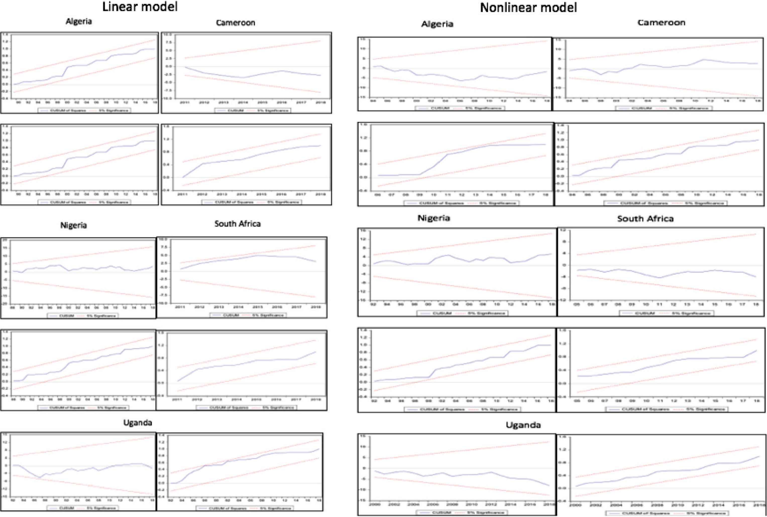
Plots of CUSUM and CUSUMSQ tests. CUSUM, plots of cumulative sum; CUSUMSQ, CUSUM of squares plots.
5.2. NARDL Estimation Results
The nonlinear model also shows the existence of a long-run association between the variables as shown in Table 7. The estimates of the positive and negative exchange rate decomposition in the nonlinear model carry meaningful and significant coefficient in almost all models except for South Africa, where the coefficient is statistically insignificant. Indeed, our result provides evidence of the J-curve effect in Algeria, Nigeria, and Uganda, amidst distinct responses of the trade balance to exchange rate shocks. This supports Bahmani-Oskooee and Fariditavana (2016), who present evidence of a nonlinear effect of real effective exchange rate on the trade balance.
| Model | Algeria | Cameroon | Nigeria | South Africa | Uganda |
|---|---|---|---|---|---|
| F-statistic | 4.333 | 6.476 | 5.555 | 3.739 | 8.452 |
| k | 4 | 4 | 4 | 4 | 4 |
| Significance level (lower–upper bound) | |||||
| 1% | 3.74–5.06 | 3.29–4.37 | 3.29–4.37 | 3.29–4.37 | 3.29–4.37 |
| 5% | 2.86–4.01 | 2.56–3.49 | 2.56–3.49 | 2.56–3.49 | 2.56–3.49 |
| 10% | 2.45–3.52 | 2.2–3.09 | 2.2–3.09 | 2.2–3.09 | 2.2–3.09 |
Bound test for Nonlinear Autoregressive Distributed Lag (NARDL) model
The results of the short-run NARDL model are provided in Table 8. The coefficient of the positive real effective exchange rate shock (REER_POS) in South Africa and Uganda are negative and statistically significant, suggesting that the J-curve hypothesis holds in the short run for the two countries. A real appreciation of the South African rand and Ugandan shilling by 1% is associated with a deterioration of trade balance by 0.28% and 1.59%, respectively. A similar outcome is observed for Nigeria, whereby a 1% depreciation of the naira exchange rate would result in a 0.8% decrease in the trade balance, suggesting that in the medium term a real depreciation worsens trade balance.
| Model | Algeria | Cameroon | Nigeria | South Africa | Uganda |
|---|---|---|---|---|---|
| Short-run estimates | |||||
| ΔLDINC | 0.453** (0.201) | –0.116 (0.113) | – | 0.566* (0.113) | –0.001 (0.087) |
| ΔLDINCt − 1 | –0.895* (0.258) | – | – | – | –0.291* (0.095) |
| ΔLDINCt − 2 | – | – | – | – | –0.509** (0.105) |
| ΔLFINC | –1.832* (0.589) | – | – | –0.280 (0.191) | –1.333* (0.344) |
| ΔLFINCt − 1 | – | – | – | – | 0.446 (0.318) |
| ΔLREER_POS | 2.045 (0.954) | 2.626* (0.386) | –0.339 (0.330) | –0.805* (0.168) | –1.594* (0.434) |
| ΔLREER_POSt − 1 | 2.508* (0.784) | 0.727*** (0.395) | –0.848** (0.386) | – | 0.446 (0.318) |
| ΔLREER_POSt − 2 | – | – | – | – | 0.914* (0.245 |
| ΔLREER_NEG | – | –0.048 (0.166) | 0.413* (0.128) | –0.228 (0.192) | –0.701* (0.244) |
| ΔLREER_NEGt − 1 | – | 0.698* (0.147) | – | – | 0.710* (0.227) |
| ΔLREER_NEGt − 1 | – | – | – | – | 0.534* (0.159) |
| ECT−1 | –0.419* (0.084) | –0.716* (0.105) | –0.938* (0.149) | –0.401* (0.078) | –0.704* (0.088) |
| Diagnostic statistics | |||||
| R2 | 0.466 | 0.658 | 0.525 | 0.692 | 0.762 |
| Adjusted R2 | 0.380 | 0.590 | 0.466 | 0.616 | 0.703 |
| Durbin–Watson stat | 1.886 | 1.806 | 2.033 | 2.055 | 2.177 |
| ARCH test | 1.185 | 0.642 | 0.432 | 0.789 | 0.303 |
| White test | 0.562 | 7.861 | 0.571 | 1.707 | 0.593 |
| RESET | 0.126 | 0.044 | 0.476 | 0.196 | 0.839 |
| Wald test long run | 2.977* | 13.184** | 1.191 | 8.580* | 9.098* |
| Wald test short run | 1.868 | 2.635* | 0.714 | 5.172* | 4.190** |
Numbers inside parentheses are standard errors.
1% significance level;
5% significance level;
10% significance level.
Short-run Nonlinear Autoregressive Distributed Lag (NARDL) model estimates
The findings also show that the coefficient of negative real effective exchange rate shock (REER_NEG) is positive and statistically significant at 1% level for Nigeria. This means that a real appreciation of the domestic currency is expected to improve trade balance by 0.41% in the short run. A plausible explanation is that Nigerian naira–US dollar exchange rate over the years has witnessed depreciation episodes mainly because of oil price volatility, inconsistent monetary policy, and misaligned exchange rates in the parallel and official markets, thereby heightening macroeconomic uncertainty and foreign exchange shortages (World Bank, 2020). The coefficient of REER_NEG for the rest of the countries is negative, which means that a real appreciation contemporaneously worsens the trade balance.
Another encouraging aspect of the results is that the ECT is negative and statistically significant in all models, suggesting that the speed of adjustment toward equilibrium following short-run deviations is quite fast. This also provides strong support for the long-run equilibrium relationship. According to Arize et al. (2017), ignoring the cointegrating relationship among variables introduces misspecification bias in the underlying dynamic framework of empirical work on estimating the J-curve effects. In Algeria, the ECT coefficient shows that about 42% of the deviation from an equilibrium path would be restored within a year. The short-run diagnostic tests support the absence of autocorrelation, model misspecification, and stable parameter estimates among other diagnostic tests.
The estimated long-run coefficients are presented for each of the countries in Table 9. The coefficient of LREER_POS is positive in all countries except South Africa but only significant for Algeria and Uganda. This suggests the existence of a long-run J-curve effect during the review period. A 1% devaluation of the domestic currency is associated with a 6.6% and 2.3% improvement of the trade balance in Algeria and Uganda, respectively, over the long run. This implies that a real depreciation of the Algerian dinar and Ugandan shilling could boost exports and improve the trade balance, which is contrary to the predictions of the J-curve hypothesis.
| Model | Algeria | Cameroon | Nigeria | South Africa | Uganda |
|---|---|---|---|---|---|
| Long-run estimates | |||||
| LDINC | 1.589 (1.161) | 0.329 (0.234) | –0.410* (0.142) | 0.132 (0.136) | 0.049 (0.139) |
| LFINC | –0.790 (1.206) | –0.303 (0.384) | 0.607*** (0.298) | 0.709** (0.298) | –0.222 (0.369) |
| LREER_POS | 6.661** (3.102) | 0.251 (0.527) | 0.108 (0.154) | –0.401 (0.576) | –2.340*** (1.252) |
| LREER_NEG | –0.591 (1.754) | –0.784*** (0.429) | 0.637* (0.183) | 0.396 (0.303) | –1.119*** (0.641) |
| C | – | 1.047 (6.551) | –6.511 (7.953) | –24.978** (11.626) | 4.304 (8.723) |
Numbers inside parentheses are standard errors.
1% significance level;
5% significance level;
10% significance level.
LREER_POS, log of positive real effective exchange rate shocks; LREER_NEG, log of negative real effective exchange rate shocks.
Long-run Nonlinear Autoregressive Distributed Lag (NARDL) model estimates
By contrast, the coefficient on the REER_NEG is negative for Cameroon and Algeria, but only significant in the former, indicating that a real appreciation of the CFA franc would worsen the country’s trade balance in the long run. Yet, the estimate is positive for Nigeria, South Africa, and Uganda, implying that real appreciation might improve trade balance in the long run.
Although the NARDL approach provides novel insights and empirical validation to the broader literature, it is not without limitations. For instance, accounting for asymmetries does not reflect the empirical regularity in African countries where depreciation spells are rife. In Nigeria, for example, the Wald test did not provide evidence of the asymmetric response of trade to real exchange rate fluctuations, which could preliminarily rule out the relevance of NARDL approach. However, it is pertinent to note that Nigeria, like other African countries, is highly resource-dependent and this magnifies its vulnerabilities to external shocks. This has not been considered in this paper but could serve as an important agenda for future studies. Furthermore, the existence of a long-run association between the variables even though the coefficients of real effective exchange rate movements are insignificant in the models indicates that the trade balance in the selected countries is more responsive to domestic and foreign income compared with the real effective exchange rate.
The empirical analysis reinforces the lack of consensus in the J-curve literature as summarized in Table 10. Neither the linear nor nonlinear models provide conclusive evidence on the effect of a devaluation on the trade balance in the selected African countries. For example, the long-run linear ARDL model shows that the J-curve effect holds for Algeria, whereas for Uganda the hypothesis contemporaneously holds in both linear and nonlinear models. The short-run J-curve hypothesis holds in South Africa and Uganda based on the nonlinear model, whereas it holds in the long-run for Algeria and Uganda. The result shows that the linear and nonlinear models are complementary, thereby making it difficult to prioritize one model over the other. Nevertheless, our findings underscore the need to model asymmetries.
| Model | Algeria | Cameroon | Nigeria | South Africa | Uganda |
|---|---|---|---|---|---|
| ARDL long run | Yes | No | No | No | No |
| ARDL short run | No | No | No | No | Yes |
| NARDL long run | Yes | No | No | No | Yes |
| NARDL short run | No | No | No | Yes | Yes |
Summary of results on the validity of the J-curve in selected countries
Similarly, Bahmani-Oskooee and Harvey (2018) and Nusair (2016) note that although empirical work on the J-curve has rapidly increased in recent years, evidence has been patchy and highly sensitive to model choice, country context, and periods. Based on our findings, the J-curve hypothesis does not fully hold for the countries considered between 1980 and 2018. This finding corroborates previous results by Bahmani-Oskooee and Gelan (2012), who did not find strong evidence of the short-run J-curve phenomenon in their study of several African countries, although their work differed from the present one in terms of the time frame and case studies. Nonetheless, our empirical results of a long-term positive effect of a real depreciation in Nigeria conform with the findings of Bahmani-Oskooee and Gelan (2012), Babatunde (2014), Bawa et al. (2018), and Igue and Oguleye (2014). By contrast, these findings do not concur with those of Akonji et al. (2013), who document the absence of a long-run relationship between the real effective exchange rates and trade balance in Nigeria. Admittedly, the differences may be traced to our decomposition of the exchange rate shocks.
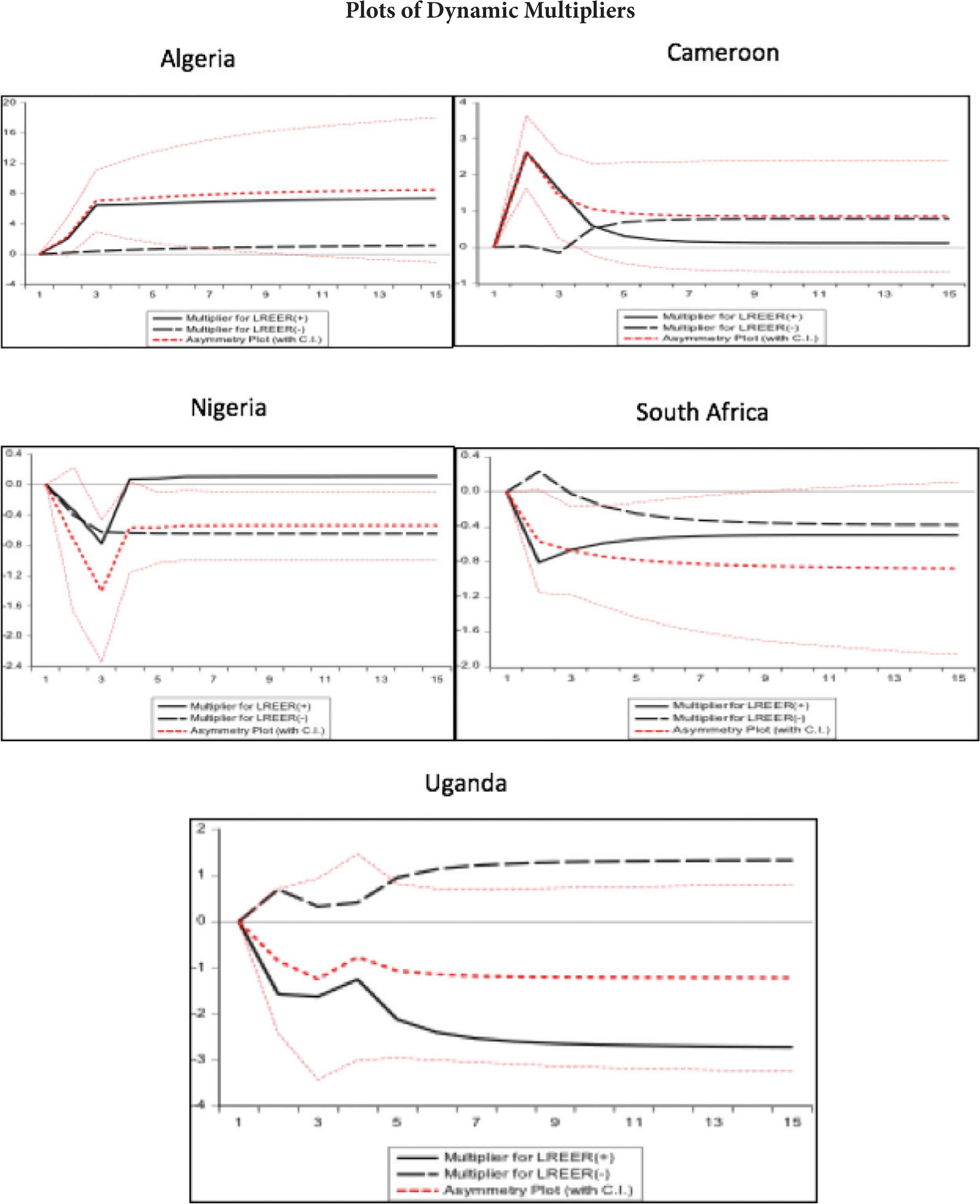
5.3. Further Checks: Dynamic Multipliers and Parameter Stability
To ascertain the adjustment of asymmetry in the long-run equilibrium following a real exchange rate appreciation or depreciation, a dynamic multiplier plot is presented in the Appendix. For most countries, the positive and negative change curves show evidence of asymmetric adjustment of the trade balance to positive and negative shocks over time. The difference between the positive and negative curves forms the asymmetry line, which represents the linear mixture of the dynamic multipliers associated with real appreciation and depreciation. The fact that a real appreciation and depreciation have an asymmetric effect on trade balance reinforces the suitability of using the NARDL in this paper. Figure 4 contains the plots of the CUSUM and CUSUMSQ tests, which are used to ascertain the stability of the model. The CUSUM tests suggest that the parameters of the models are stable, given that the recursive residuals are located within the two critical bounds at the 5% significance level.
6. CONCLUSION
The relationship between exchange rate and trade balance has attracted significant attention among scholars and policymakers. The general consensus is that the J-curve holds in African countries especially in the context of linear models. Contrary to this notion, we argue that exchange rate asymmetries could matter, and this largely depends on the country or region considered. Using linear and nonlinear ARDL models, we assessed the existence of the J-curve hypothesis in five African countries and found that it does not completely hold in any of the countries between 1980 and 2018. Specifically, the linear model showed that the short-run J-curve effect holds contemporaneously in Uganda and in Algeria over the long term. However, the nonlinear model indicated that the short-run J-curve holds for South Africa and Uganda, whereas evidence of long-run J-curve effects was found in Algeria and Uganda. The results make a case for modeling asymmetries as the nonlinear model performed relatively better. These findings should be viewed with caution as general inferences cannot be drawn for Africa as a whole because only five countries were analyzed. In addition to the use of a panel NARDL covering more countries, future studies could also consider other potential control variables that could explain the dynamics of the trade balance. The finding that exchange rate devaluations do not exert a clear and significant influence on the trade balance has important policy implications. There is a need for policymakers to address structural imbalances in the economy to leverage on the exchange rate and trade policies to improve the trade balance. This includes ensuring that multiple exchange rate windows are eliminated to minimize speculative activities and spur competitiveness. More diversified and high value-added export-oriented sectors could be considered to sustainably close the current account deficit.
CONFLICTS OF INTEREST
The authors whose names are listed immediately below certify that they have NO affiliations with or involvement in any organization or entity with any financial interest, or non-financial interest in the subject matter or materials discussed in this manuscript.
AUTHORS’ CONTRIBUTION
MS and AI contributed in abstract, background of the study and conclusion. MS contributed in introduction, methodology, writing, proofreading and editing, charts and also in discussion of findings. AI contributed in literature review and references.
FUNDING
The authors (Mohammed Shuaibu and Abdulrasheed Isah) received no financial support for the research, authorship, and/or publication of this article.
ACKNOWLEDGMENTS
The authors appreciate the editorial team and anonymous reviewers for their very helpful comments and feedback which helped to improve the paper.
APPENDIX
Footnotes
The volume effect would improve trade balance by boosting exports because domestic goods become cheaper after a real depreciation, whereas the price effect could worsen it as imports become more expensive.
In addition to the possibility of simultaneously testing the long and short-run nonlinearities through the positive and negative partial sum decompositions of regressors, it also offers the possibility of quantifying the respective responses of the dependent variable to positive and negative shocks of the regressors from the asymmetric dynamic multipliers (Arize et al., 2017).
REFERENCES
Cite this article
TY  - JOUR
AU  - Mohammed Shuaibu
AU  - Abdulrasheed Isah
PY  - 2020
DA  - 2020/12/29
TI  - Exchange Rate Dynamics and Trade Balance in Selected African Countries
JO  - Journal of African Trade
SP  - 69
EP  - 83
VL  - 7
IS  - 1-2
SN  - 2214-8523
UR  - https://doi.org/10.2991/jat.k.201218.001
DO  - 10.2991/jat.k.201218.001
ID  - Shuaibu2020
ER  -