
Comparison of Predictive Models and Impact Assessment of Lockdown for COVID-19 over the United States
Centre for Environmental Studies, Department of Geography, Geoinformatics and Meteorology, University of Pretoria, Pretoria 0002, South Africa
- DOI
- 10.2991/jegh.k.210215.001How to use a DOI?
- Keywords
- COVID-19; USA; INGARCH; negative binomial; ARIMA; lockdown policy
- Abstract
The novel Coronavirus Disease 2019 (COVID-19) remains a worldwide threat to community health, social stability, and economic development. Since the first case was recorded on December 29, 2019, in Wuhan of China, the disease has rapidly extended to other nations of the world to claim many lives, especially in the USA, the United Kingdom, and Western Europe. To stay ahead of the curve consequent of the continued increase in case and mortality, predictive tools are needed to guide adequate response. Therefore, this study aims to determine the best predictive models and investigate the impact of lockdown policy on the USA’ COVID-19 incidence and mortality. This study focuses on the statistical modelling of the USA daily COVID-19 incidence and mortality cases based on some intuitive properties of the data such as overdispersion and autoregressive conditional heteroscedasticity. The impact of the lockdown policy on cases and mortality was assessed by comparing the USA incidence case with that of Sweden where there is no strict lockdown. Stochastic models based on negative binomial autoregressive conditional heteroscedasticity [NB INGARCH (p,q)], the negative binomial regression, the autoregressive integrated moving average model with exogenous variables (ARIMAX) and without exogenous variables (ARIMA) models of several orders are presented, to identify the best fitting model for the USA daily incidence cases. The performance of the optimal NB INGARCH model on daily incidence cases was compared with the optimal ARIMA model in terms of their Akaike Information Criteria (AIC). Also, the NB model, ARIMA model and without exogenous variables are formulated for USA daily COVID-19 death cases. It was observed that the incidence and mortality cases show statistically significant increasing trends over the study period. The USA daily COVID-19 incidence is autocorrelated, linear and contains a structural break but exhibits autoregressive conditional heteroscedasticity. Observed data are compared with the fitted data from the optimal models. The results further indicate that the NB INGARCH fits the observed incidence better than ARIMA while the NB models perform better than the optimal ARIMA and ARIMAX models for death counts in terms of AIC and root mean square error (RMSE). The results show a statistically significant relationship between the lockdown policy in the USA and incidence and death counts. This suggests the efficacy of the lockdown policy in the USA.
- Copyright
- © 2021 The Authors. Published by Atlantis Press International B.V.
- Open Access
- This is an open access article distributed under the CC BY-NC 4.0 license (http://creativecommons.org/licenses/by-nc/4.0/).
1. INTRODUCTION
The novel Coronavirus Disease 2019 (COVID-19) recently gained attention as the virus continues to claim more lives globally. The disease hastily spread from Wuhan to further China provinces and other nations worldwide. Currently (as of August 10, 2020), more than 19.8 million cases have been confirmed with about 12.1 million recovered and 732,000 related deaths across the globe, as stated by the Johns Hopkins virus dashboard. At the beginning of the epidemic, elderly people were more susceptible to COVID-19 [1]. As the epidemic progressed, an increase in the number of cases among people between 45 and 64 years was recorded, as well as an upsurge in the number of cases among individuals, especially individuals between 18 and 44 years [2]. Reports also show that the cases are 2.6 times higher on Black/African American and 2.8 times higher on Hispanic/Latino individuals. Furthermore, COVID-19 induced death is nine times lower on 0–4 years old children and 630 times higher on 85+ years old adults [3]. The various signs associated with COVID-19 are fever, dry cough, short breath, and breathing difficulties. COVID-19 poses a severe threat to the health of individuals worldwide; on January 30, 2020, the World Health Organization declared a universal health emergence on COVID-19 [4,5].
On January 21, 2020, the COVID-19 index case was confirmed in the USA. Roughly a month after that (February 29, 2020), the first death was reported in Washington state. As of August 10, 2020, the USA has confirmed about 4.9 million cases and over 161,284 related deaths. At least 229,073 of those cases occurred in New York City, 184,429 in New Jersey, 120,711 in Massachusetts, 193,998 in Illinois, 118,092 in Pennsylvania, 96,191 in Michigan, and 545,787 in California [6].
At the beginning of the COVID-19 pandemic, a model was developed by the National Institute of Allergy and Infectious Diseases to predict the total sum of mortality cases. Although the model was reviewed with updated data by March ending, some COVID-19 models, including one from the Institute for Health Metrics and Evaluation (IHME), had predicted that despite some preventive measures such as stay-indoors and additional measures of social distance, 200,000 persons living in the USA might eventually die of this virus. As of April 7, model by IHME predicted 60,415 mortality cases in the USA due to COVID-19. The model anticipated that the daily mortality cases will peak on April 12 with 2212 related deaths on that day [7].
Lauer et al. [8] projected the span of the incubation time of COVID-19 and then presented its consequences for community health. Lauer et al. [8] argued that the median incubation period for 2019-nCoV is approximately 5 days, this is similar to the incubation time of severe acute respiratory syndrome. If infection ensues at the beginning of monitoring, the authors also argued that in 10,000 cases, 101 will show symptoms afterward 2 weeks of effective monitoring or seclusion. In another development, Jiang et al. [9] discussed some developments in research and production of deactivating antibodies used in the deterrence and cure of 2019-nCoV infection and other human coronaviruses. Zhang et al. [2] applied the Bayesian technique to determine the dynamics of the net reproduction number of provinces in China. Fanelli and Piazza [10] analysed COVID-19 cases over China, Italy, and France using a simple susceptible-infected-recovered-deaths model. Makinde et al. [11] analysed daily COVID-19 mortality rates in African countries using a generalized estimating equation and showed that there are significant monotone trends in the daily COVID-19 incidence and mortality counts of many countries in Africa as well as a positive weak linear relationship amid the daily reported COVID-19 cases and African countries’ population. Hafner [12] fitted spatial autoregressive models to the number of newly infected people in some countries by finding strong spillovers and distances between such that forecast error variances of many countries can be explained by structural innovations of other countries. However, this model did not consider the effect of over-dispersion of the number of newly infected people. Yue et al. [13] considered an early warning and risk identification for COVID-19 and suggested some solutions and recommendations, which include institutional cooperation, and to inform national and international policymakers.
Benvenuto et al. [14] formulated an Autoregressive Integrated Moving Average (ARIMA) model of order p, d, and q on the COVID-19 epidemic dataset. Similarly, Singh et al. [15] applied discreet wavelet decomposition and ARIMA model to COVID-19 death cases in some countries. However, the ARIMA (p,d,q) model may not be appropriate for count data, especially when the data are over-dispersed. This study aims to determine the best fitting predictive models for the USA’ COVID-19 and investigate the impact of lockdown policy on the USA’ COVID-19 incidence and mortality. The study targets the best fitting model for predictive and inferential purposes. Distributions of age and race for incidence and death cases are presented to identify race and age group with high vulnerability to COVID-19. Overdispersion of the COVID-19 daily incidence cases in the USA is considered with the purpose of formulating a predictive model for the data. In particular, a negative binomial integer generalized autoregressive conditional heteroscedasticity models of orders p and q, and a negative binomial regression model are formulated for the USA’ daily COVID-19 incidence and death counts from January 21 to August 8, 2020. The negative binomial integer generalized autoregressive conditional heteroscedasticity models and a negative binomial regression model are considered to handle overdispersion and autoregressive conditional heteroscedasticity exhibited by the USA’ daily COVID-19 incidence and death counts. Also, the impact of lockdown policy in the USA is considered with Sweden where there is no strict lockdown policy.
2. MATERIALS AND METHODS
2.1. Data
Data analysed in this study comprise of the USA daily count of COVID-19 reported from January 21 to August 8, 2020. The daily reported incidence cases in this study have been sourced from the Centre for Disease Control (CDC) and the European CDC (ECDC). Although the data do not include cases amid individuals sent back to the USA from China and Japan, it embraces together established and probable positive COVID-19 cases told to the CDC or verified at state and indigenous public health departments since January 21, 2020 [16,17].
2.2. Models
2.2.1. Negative binomial integer autoregressive conditional heteroscedasticity (NB INGARCH) model
It is important to investigate whether the data are random, linear, contain structural breaks and exhibit autoregressive conditional heteroscedasticity. The autoregressive models can only be applied on correlated (non-random) and linear data. The Ljung–Box test will be used to investigate if the COVID-19 incidence counts are random or autocorrelated. Tsay’s test for nonlinearity is used to investigate the nonlinearity of the COVID-19 incidence data. Teraesvirta’s neural network test investigates if the time series is linearity in the mean. Also, structural break tests help to investigate whether there is a significant change in the COVID-19 incidence cases while the Chow test will be applied to test if there are structural breaks in the data. McLeod–Li test may be applied to test the null hypothesis that the data do not exhibit autoregressive conditional heteroscedasticity effects. COVID-19 incidence counts are said to exhibit autoregressive conditional heteroscedasticity if mean incidence cases increase with time.
A predictive model such as negative binomial integer autoregressive conditional heteroscedasticity model is used on a time series that exhibit overdispersion and conditional heteroscedasticity. Suppose Xt is a daily COVID-19 incidence count which is distributed as a negative binomial with parameters μt and γ, where γ is an overdispersion parameter, which measures how close the mean of the series is to the variance. The parameter μt is the mean of the distribution of Xt at time t. Suppose Xt has a conditional heteroscedasticity effect, a predictive model based on negative binomial integer autoregressive conditional heteroscedasticity is formulated for daily USA COVID-19 incidence count. The negative binomial integer autoregressive conditional heteroscedasticity model is formulated to handle overdispersion and autoregressive conditional heteroscedasticity of the incidence count. The negative binomial integer autoregressive conditional heteroscedasticity model of order p and q, denoted by NB INGARCH (p,q), is defined as
2.2.2. The negative binomial regression model
Following some recent studies [19], a negative binomial regression model of the form loge(E(Y) = β0 + β1X1 + β2X2 + ... + βpXp + ɛ may be formulated for the total number of death cases based on incidence cases. However, it is assumed that incidence precedes mortality. Also, daily incidence cases contain some outlying observations and its variability could be very high in many situations. Consequently, logarithmic transformation of the daily incidence cases is needed to reduce the variability of data. Hence, in this work, Negative Binomial (NB) regression model of the form:
2.2.3. The autoregressive integrated moving average model with exogenous variables
Similar to Abiodun et al. [20] and Makinde and Abiodun [21], an ARIMA (p,d,q) model with exogenous variables can be formulated for the number of COVID-19 death cases. In fitting ARIMA (p,d,q) model with exogenous variables for the number of COVID-19 death cases, the optimal ARIMA model is chosen as the one with least AIC in a class of ARIMA models of various values of p, d, and q, where the exogenous variable is the daily incidence cases at lags 0–14. The ARIMA (p,d,q) model with exogenous variables is formulated as
2.2.4. Wilcoxon rank-sum test
Wilcoxon rank-sum test can be used to check whether two independent samples were selected from populations having the same distribution. The Wilcoxon rank-sum test with continuity correction is applied to test if incidence rates in the USA and Sweden are significantly different. For a fixed significance level α, the test statistic is computed by combining two samples and rank all observations from smallest to largest while keeping track of the sample to which each observation belongs. The Wilcoxon rank-sum test concludes that the two countries are not identical in terms of their COVID-19 incidence rate if the p-value of the test is less than the value of α.
3. RESULTS AND DISCUSSION
3.1. Analysis of the USA’ COVID-19 Incidence Cases
The incidence of COVID-19 was computed from the prevalence and presented in Figure 1. It could be observed that there is an upward trend in COVID-19 incidence in the USA. Figure 2 presents the distribution of race on the USA’ reported incidence and death cases. It is shown from Figure 2 that the race “White, non-Hispanic”, “Hispanic/Latino” and “Black, non-Hispanic” are more vulnerable to COVID-19 as of August 8, 2020.
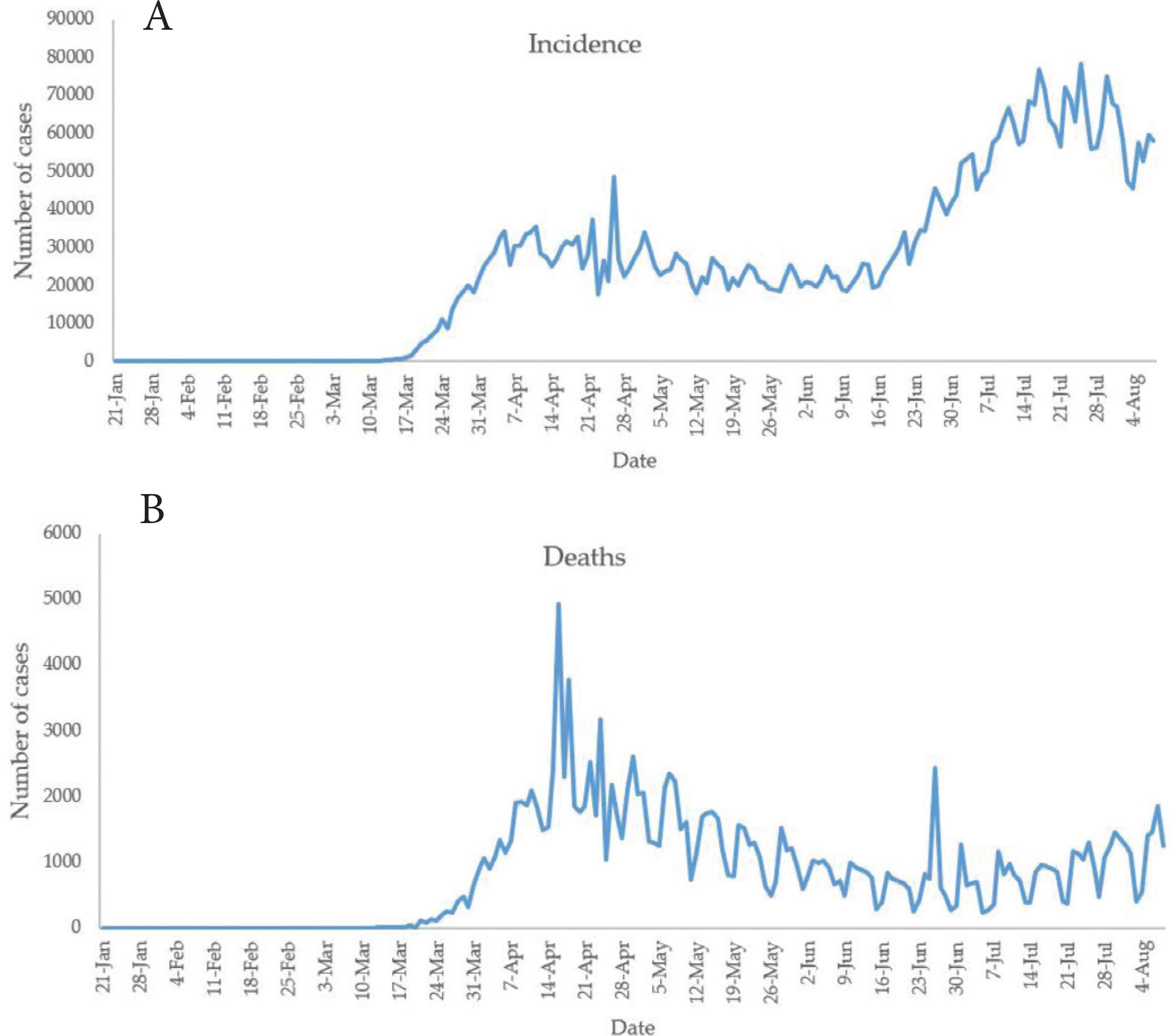
The plot of counts of COVID-19 (A) incidence and (B) death cases in the USA.
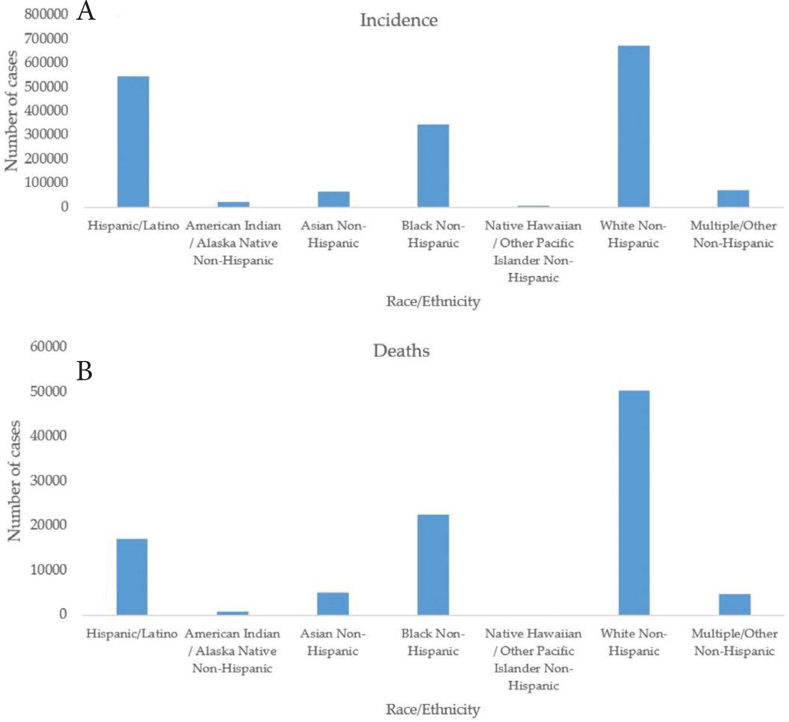
Race distribution of COVID-19 (A) incidence and (B) death cases in the USA.
Figure 3 presents the distribution of age groups on the USA’ reported cases. It is shown from the figure that the age groups 18–44 and 50–64 are the most vulnerable to the COVID-19. The age groups 50 and above are at higher risk of COVID-19 mortality.
Age groups distribution of COVID-19 (A) incidence and (B) deaths in the USA.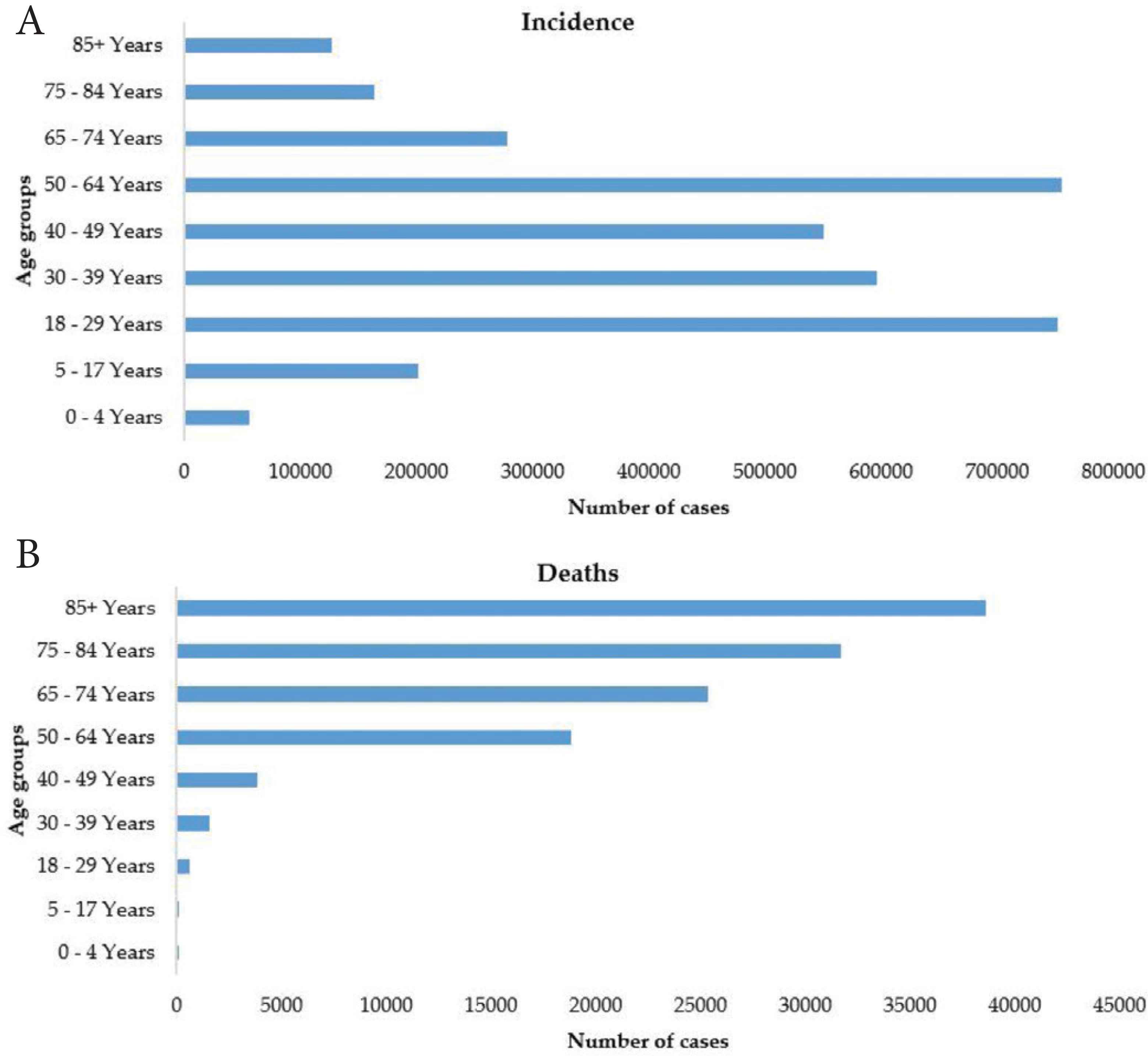
In investigating whether the data are random, linear, contain structural breaks and exhibit autoregressive conditional heteroscedasticity, the Ljung–Box test confirms that the COVID-19 incidence counts are autocorrelated (p = 0.000). Tsay’s test for nonlinearity showed that the daily incidence cases are linear and follow some autoregressive (AR) process (p = 0.000). Also, Chow test (p = 0.000) confirms a structural break in the daily incidence cases. Teraesvirta’s neural network test showed that the daily incidence cases are linearity in the mean. McLeod–Li test rejects the null hypothesis and concludes that there is an autoregressive conditional heteroscedasticity in the USA COVID-19 incidence data (Maximum p = 0.000) at a 5% level of significance.
There is a significant upward trend in the COVID-19 daily incidence of the USA from January 21 to April 11, 2020 (p = 0.000), a downward trend from April 12 to June 10, 2020 (p = 0.000), and an upward trend from June 11 to July 30, 2020 (p = 0.000). The first-order autocorrelation of daily reported incidence cases of the USA is positive (0.965). Low-order autocorrelation of COVID-19 incidence [12] is predominantly positive with cycles of 2–5 days in the USA. There is the presence of short-term cycles in the number of incidence and death cases. The short-term cycles are between 2 and 5 days in the USA.
It was observed that there are a few days with zero counts from January 21, 2020 to February 27, 2020 (Figure 1). Also, there are non-zero counts from February 28, 2020 to August 8, 2020. The NB-INGARCH (p,q) model for some values of p and q is formulated for the USA’ daily COVID-19 incidence count from January 21, 2020 to August 8, 2020. Comparing the AIC values of NB-INGARCH (p,q) model for some values of p and q, NB-INGARCH (2,2) model has the least AIC values (AIC = 3543.522). The measure of dispersion of the data is shown in terms of the estimate of γ (0.2468). The closer the estimate of γ from 0, the more overdispersed is the data (that is, the greater is its variance than its mean). The mathematical expression for the predictive model for the incidence count is
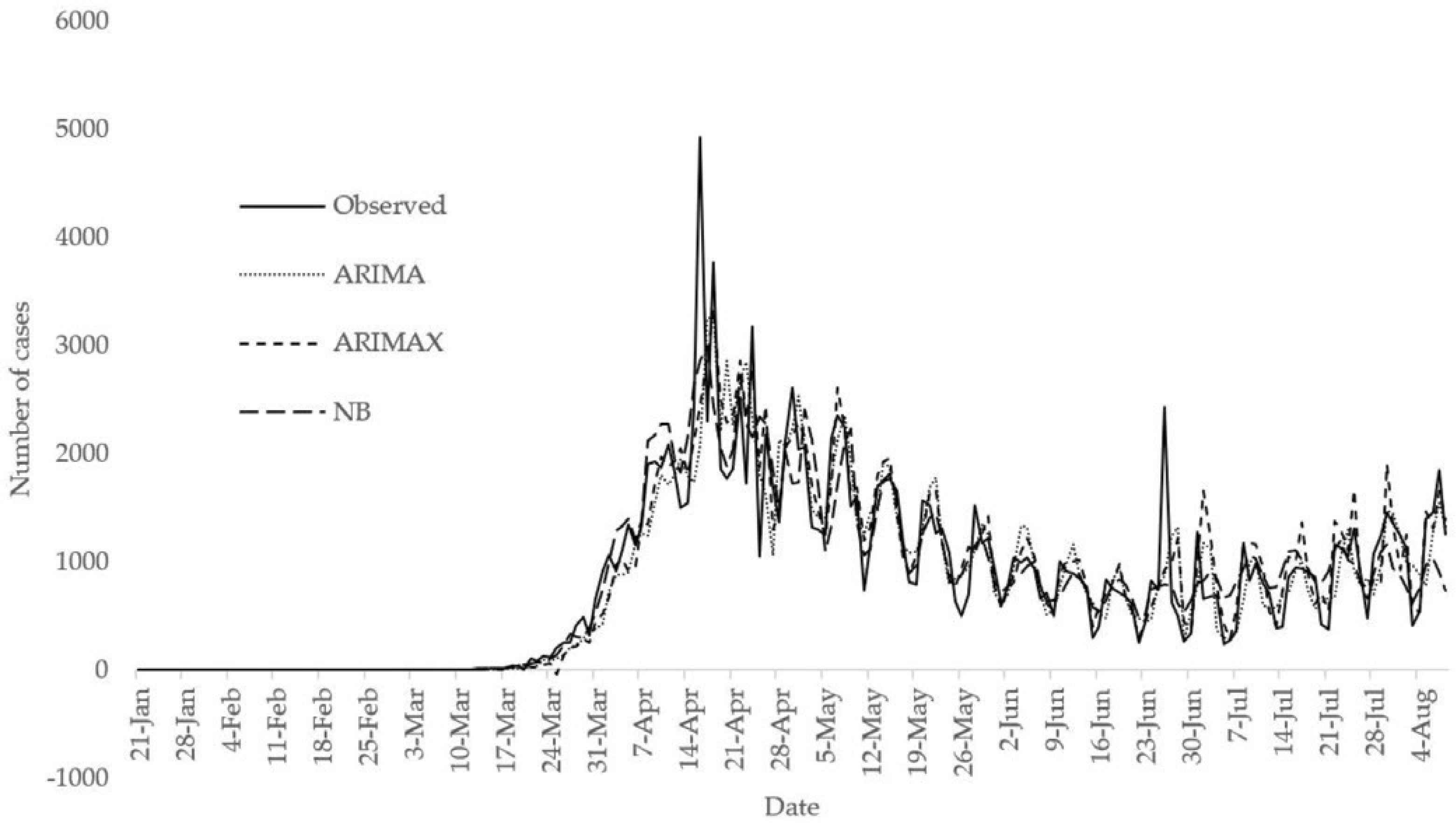
To demonstrate the performance of ARIMA (p,d,q) on the count data following [9], an ARIMA model of various orders were formulated for the USA daily COVID-19 incidence cases. The optimal model was identified as ARIMA (1,1,1) model with drift based on the least AIC value. The AIC value of the optimal ARIMA model is 3948.93 while the AIC value of the optimal NB INGARCH model is 3543.522+. Comparing the AIC values of ARIMA (1,1,1) model with drift and NB-INGARCH (2,2) model, it can be inferred that the NB-INGARCH (2,2) has better predictive power. Figure 4 presents a comparison between observed counts and fitted values from ARIMA (1,1,1) model with drift and NB-INGARCH (2,2) model. It can be observed from the figure that both optimal ARIMA and NB INGARCH models fit the data well. However, the optimal NB INGARCH model over-fits the first data point. Comparing the two models in terms of AIC, the optimal NB INGARCH model achieves lower AIC value than the optimal ARIMA model. Hence, the NB INGARCH model exercised superior performance over the ARIMA model.

Comparison between observed counts, fitted values from optimal NB INGARCH (2,2) model and fitted values from optimal ARIMA (1,1,1) model with drift.
3.2. Analysis of the USA’ COVID-19 Death Cases
There is a significant upward trend in the COVID-19 daily death cases of the USA from January 21 to April 16, 2020 (p = 0.000), a significant downward trend from April 17 to June 20, 2020 (p = 0.000) and significant upward trend from June 21 to August 8, 2020 (p = 0.000).
The need for the logarithmic transformation of Xt in Equation (2) can be observed from the variability of Xt. The variance of Xt is 470,035,583. This is shown in the boxplot in Figure 5A. The variance of the natural logarithm of (Xt + 1) is 16.4609. The value 1 is added to Xt before taking the natural logarithm because there are days with no reported cases. This is shown in the second boxplot in Figure 5B.
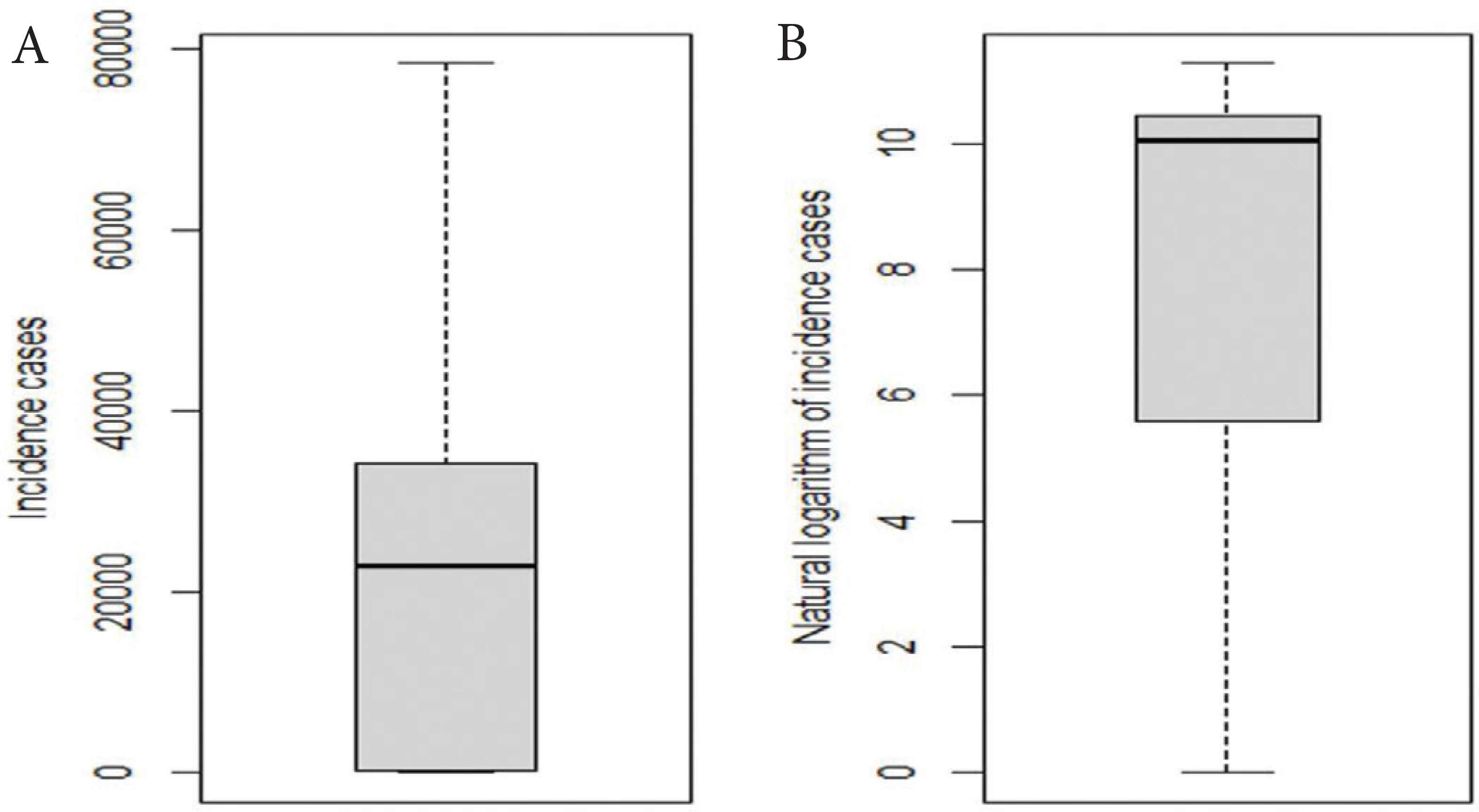
Boxplot of (A) COVID-19 incidence cases and (B) the natural logarithm of COVID-19 incidence cases in the USA.
The NB model in Equation (2) was formulated for the number of COVID-19 death cases as a function of the number of reported cases at some lag values. The AIC value for the model [Equation (2)] is 2223.842. The model with the least AIC (AIC = 2218.944) excludes the number of reported cases at lags 1, 3, 8, 10, 11, and 14. The coefficient of natural logarithms of the number of COVID-19 reported cases at lags 4 and 5 predicting the total number of new deaths is not statistically significant at a 5% level of significance. Table 1 shows the estimates of coefficients of NB regression model for the number of COVID-19 death cases in the USA. Suppose Wt−i denote loge(Xt−i + 1), the number of death cases in the USA increases by a factor of 1.3594, 1.3118, 1.5326, 1.3145, and 1.4145 for a 1-unit increase in Wt at lags 0, 6, 7, 12, and 13 respectively when other variables are held constant. The number of death cases in the USA increases by a factor of 0.9841, 0.6805, and 0.6907 for a 1-unit decrease in t and Wt at lags 2 and 9 respectively when other variables are held constant.
| Predictor variables | Estimate | Std. error | z-value | Pr (>|z|) | Confidence interval |
|---|---|---|---|---|---|
| t | −0.016 | 0.0009 | −17.089 | <2.22 × 10⁻¹⁶*** | (−0.0178, −0.0142) |
| log(Xt + 1) | 0.3070 | 0.1028 | 2.987 | 0.0028** | (0.1056, 0.5085) |
| log(Xt−2 + 1) | −0.3849 | 0.1312 | −2.933 | 0.0034** | (−0.6421, −0.1277) |
| log(Xt−6 + 1) | 0.2714 | 0.1210 | 2.243 | 0.0249* | (0.0343, 0.5086) |
| log(Xt−7 + 1) | 0.4269 | 0.1244 | 3.431 | 0.0006*** | (0.1830, 0.6708) |
| log(Xt−9 + 1) | −0.370 | 0.1258 | −2.942 | 0.0033** | (−0.6166, −0.1235) |
| log(Xt−12 + 1) | 0.2735 | 0.0974 | 2.809 | 0.0050** | (0.0827, 0.4643) |
| log(Xt−13 + 1) | 0.3468 | 0.0859 | 4.039 | 5.37 × 10⁻⁵*** | (0.1785, 0.5151) |
Significant codes:
0.001;
0.01;
0.05 [Dispersion parameter for negative binomial (7.7651) family taken to be 1].
Null deviance: 687894.68 on 187 degrees of freedom. Residual deviance: 227.69 on 179 degrees of freedom. AIC, Akaike information criterion: 2220.
Estimates of coefficients of the NB model for the number of COVID-19 death cases
It is important to investigate whether the residuals of the fitted model are random [21]. The Ljung–Box test is used. The Ljung–Box test shows that the residuals of the fitted NB model are random (p = 0.6600). Also, an ARIMA (p,d,q) model with exogenous variables is formulated for the number of COVID-19 death cases. The optimal model is ARIMA (3,1,3). The Ljung–Box test is used to check if the residuals of this model are random. The Ljung–Box test implies that the residuals of the fitted ARIMA model with exogenous variables are random (p = 0.9288).
It is also possible to fit ARIMA model without exogenous variables. The optimal ARIMA model without exogenous variables is ARIMA (3,1,2). The use of exogenous variables is better in formulating ARIMA model for the USA COVID-19 death cases because the AIC value and RMSE of the optimal ARIMA model with exogenous variables are 2911.15 and 311.3858 while the AIC value and RMSE of the optimal ARIMA model without exogenous variables are 2946.83 and 368.4422, respectively (Table 2). Figure 6 shows the comparison between observed counts and fitted values from Negative Binomial (NB) regression model, optimal ARIMA (3,1,3) model with exogenous variables (denoted by ARIMAX) and optimal ARIMA (3,1,2) model. The NB model performs better than the optimal ARIMA and ARIMAX models in terms of AIC and RMSE. Also, the NB model fits the observed death counts well. Figure 7 presents the comparison of predicted incidence and death cases from August 9 to October 8, 2020 with the observed from ECDC.
| Predictor | φt−1 | φt−2 | φt−3 | ∈t−1 | ∈t−2 | ∈t−3 | –Xt |
| Estimate | 0.759 | −0.385 | −0.442 | −1.549 | 1.219 | −0.309 | 0.023 |
| S.E | 0.104 | 0.127 | 0.092 | 0.111 | 0.166 | 0.109 | 0.006 |
| Predictor | Xt−1 | Xt−2 | Xt−3 | Xt−4 | Xt−5 | Xt−6 | Xt−7 |
| Estimate | −0.015 | −0.003 | −0.015 | −0.016 | 0.008 | −0.004 | 0.008 |
| S.E | 0.006 | 0.007 | 0.006 | 0.007 | 0.007 | 0.007 | 0.007 |
| Predictor | Xt−8 | Xt−9 | Xt−10 | Xt−11 | Xt−12 | Xt−13 | Xt−14 |
| Estimate | 0.022 | −0.003 | 0.003 | 0.023 | −0.003 | 0.001 | 0.01 |
| S.E | 0.007 | 0.007 | 0.007 | 0.007 | 0.007 | 0.007 | 0.007 |
Estimates of coefficients of the optimal ARIMA model with exogenous variables for the number of death cases in the USA
Comparison between observed counts, fitted values from NB, optimal ARIMAX and optimal ARIMA models.

Comparison of predicted values with observed values from August 9 to October 8, 2020.
3.3. Examining the Effect of Lockdown on the Incidence Cases in the USA
To account for the efficiency of lockdown policy in the USA, the incidence rate in Sweden [17], where there is no strict lockdown, is compared with that of the USA (Figure 8). The incidence rate is calculated as the ratio of incidence to the country’s population multiply by 100. The population of the USA is taken as 329,064,917 while that of Sweden is 10,230,185 [17]. It can be seen from the figure that there are upward trends in the daily incidence rate of Sweden from February 1 to June 30, 2020 (p = 0.000), and a downward trend from July 1 to August 8, 2020 (p = 0.3453). It can also be seen that there are upward trends in the daily death rate of Sweden from February 1 to April 25, 2020 (p = 0.000) and downward trend from April 26 to August 8, 2020 (p = 0.000). The mean daily incidence rate from the first incidence in Sweden is 0.00424 while that of the USA is 14.378. The mean daily death rate from the first incidence in Sweden is 0.00035 while that of the USA is 0.00024. Wilcoxon rank-sum test was used to investigate if there is a statistically significant difference between daily incidence rates in the two countries. The test shows that there is a statistically significant difference between the daily incidence rates in the two countries (p = 0.000). The Wilcoxon rank-sum test further shows that there is no statistically significant difference between the daily death rates in the two countries from the day of the first incidence to August 8, 2020 (p = 0.8922). The lockdown policies in the USA were relaxed at different dates by each state. All the states relaxed the lockdown policies before June 7 except New Jersey, which relaxed the lockdown policies on June 9. Figure 8 presents the plots of daily incidence rates and death rates in the USA and Sweden from January 21 to June 7, 2020, accounting for efficiency of lockdown policy. It is shown in the figure that daily incidence rates are higher in the USA than in Sweden between March 22 and June 3, 2020, and lower daily incidence rates in the USA than in Sweden in other days. The daily death rates are higher in Sweden than in the USA most of the days from January 21 to June 7, 2020.
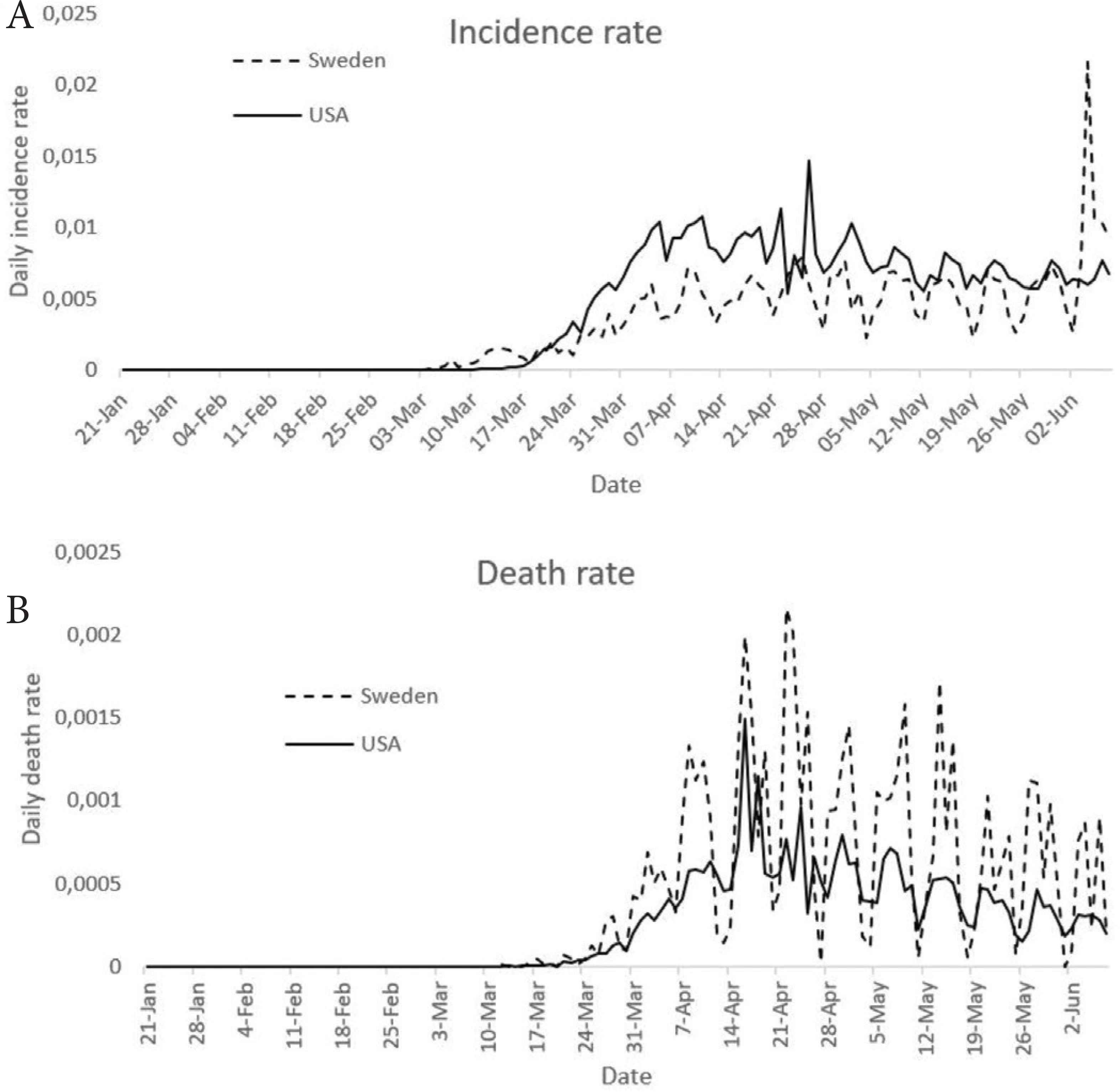
Comparison of incidence rates and death rates in the USA and Sweden, accounting for efficiency of lockdown policy.
Consequentially, lockdown policies in the USA, which aimed at reducing the incidence rates seem to yield profound results. It is observed that higher incidence rates are recorded in Sweden in some of the days under study compared to the USA. However, several factors can contribute to this. The populations of both countries differ, with a higher population in the USA. Jiang and Luo [22] observed a positive relationship between country’s population and incidence cases. Makinde et al. [11] identified population as a driver of spread of COVID-19. Due to the large population in the USA, the impact of lockdown seems less significant on the transmission in the USA when compared to that of Sweden. However, this analysis does not capture how different incidence and mortality numbers would have been, had the lockdown in the USA started early.
Comparing the daily incidence rates and death rates of the USA before and after June 7, it was found that the mean daily incidences before and after relaxing lockdown policies are 0.0042 and 46.6032, respectively. The Wilcoxon rank-sum test shows that the daily incidence rates before relaxing lockdown policies are lower than the daily incidence rates after relaxing lockdown policies (p = 0.000). This implies that the incidence rates grow exponentially after the lockdown policies were relaxed in the USA. Similarly, the death rates in the USA grow since June 7, indicating the effectiveness of the USA lockdown policies.
Recent work by counterfactual simulations [23] suggests that if non-pharmaceutical interventions (stay at home, social distancing, use of a mask), had been implemented just between 1 and 2 weeks earlier, a substantial number of incidence cases and mortality cases could have been prevented. Specifically [23], nationwide, 61.6% (between 54.6% and 67.7% at 95% confidence interval) of reported infections and 55.0% (between 46.1% and 62.2% at 95% confidence interval) of reported mortality cases as of May 3, 2020, could have been circumvented if the same control measures had been implemented just 1 week earlier.
4. CONCLUSION
In this study, the negative binomial integer autoregressive conditional heteroscedasticity models of various orders are presented for the USA daily COVID-19 incidence count from January 21 to August 8, 2020, to find an optimum model from a class of models. This is to find the best fitting model for predictive and inferential purposes. The incidence count was found to be autocorrelated, linear, and had a structural break. Also, the data exhibits autoregressive conditional heteroscedasticity. The optimal NB INGARCH model was found to be the best model based on its comparison with the observed data and lower AIC and RMSE, which indicates that the model fits the data reasonably well. In literature, ARIMA model of order p, d, and q was used on COVID-19 data. However, appropriateness of ARIMA for modelling over-dispersed count data is questionable.
A negative binomial model, an ARIMA model with exogenous variables and without exogenous variables were formulated for COVID-19 death cases in the USA. The three models fit the data well. In terms of AIC, the negative binomial model performed better than others. The inclusion of time index in the negative binomial model was aimed at improving the model. The ARIMA model with exogenous variables performs well than when exogenous variables were excluded. The NB INGARCH (5,3) model was identified to be the optimal model for fitting number of incidence cases while negative binomial model as the optimal model for fitting number of death cases.
Comparing the daily incidence and death rates in the USA with Sweden, the daily death rates in the USA are lower than that of Sweden in some days, while consistently lower in many days. It can be inferred that the effectiveness of lockdown in the USA was profound over the study period.
CONFLICTS OF INTEREST
The authors declare they have no conflicts of interest.
AUTHORS’ CONTRIBUTION
OSM conceived the study design and framework. AMA and OOO performed data cleaning. OSM, AMA and GJA conducted the statistical model and data analysis. OSM, GJA and OOO wrote the original manuscript. AMA and AA review and edited the manuscript. All authors read and approved the final manuscript.
FUNDING
No financial support was provided.
ACKNOWLEDGMENTS
The authors acknowledge the support of the University of Pretoria Institute for Sustainable Malaria Control (UP ISMC) and Malaria Research Control (MRC) collaborating centre for malaria research, South Africa.
ETHICAL APPROVAL AND CONSENT TO PARTICIPATE
No individual person data is included in this study.
Footnotes
Data availability statement: The COVID-19 data reported in this manuscript have been sourced from the Centers for Disease Control and Prevention: Cases of Coronavirus Disease (COVID-19) in the U.S. Available from: https://www.cdc.gov/coronavirus/2019-ncov/index.html.
REFERENCES
Cite this article
TY  - JOUR
AU  - Olusola S. Makinde
AU  - Abiodun M. Adeola
AU  - Gbenga J. Abiodun
AU  - Olubukola O. Olusola-Makinde
AU  - Aceves Alejandro
PY  - 2021
DA  - 2021/02/22
TI  - Comparison of Predictive Models and Impact Assessment of Lockdown for COVID-19 over the United States
JO  - Journal of Epidemiology and Global Health
SP  - 200
EP  - 207
VL  - 11
IS  - 2
SN  - 2210-6014
UR  - https://doi.org/10.2991/jegh.k.210215.001
DO  - 10.2991/jegh.k.210215.001
ID  - Makinde2021
ER  -