
The (N + 1)-Dimensional Burgers Equation: A Bilinear Extension, Vortex, Fusion and Rational Solutions
- DOI
- 10.2991/jnmp.k.200922.004How to use a DOI?
- Keywords
- The (N + 1)-dimensional Burgers system; bilinear formulation; generalized Cole-Hopf transformation; vortex solutions; multiple fusion solutions; rational solutions
- Abstract
In this paper, by introducing a fractional transformation, we obtain a bilinear formulation for the (N + 1)-dimensional Burgers equation. Such a formulation constitutes a bilinear extension to the (N + 1)-dimensional Cole-Hopf transformation between the (N + 1)-dimensional Burgers system and generalized heat equation. As applications of the bilinear extension to the Cole-Hopf transformation, four types of physically interesting exact solutions are constructed, which contain vortex solutions, multiple fusions, rational solutions and triangular rational solutions. The behaviors of these solutions are analyzed and simulated. Interestingly, the type of fusion solutions has recently found applications in organic membrane, macromolecule material, even-clump DNA, nuclear physics and plasmas physics et al.
- Copyright
- © 2020 The Authors. Published by Atlantis Press B.V.
- Open Access
- This is an open access article distributed under the CC BY-NC 4.0 license (http://creativecommons.org/licenses/by-nc/4.0/).
1. INTRODUCTION
Exact solutions to Partial Differential Equations (PDEs) are important. Not only because they can serve as useful tools to test the effectiveness of numerical algorithms of the PDEs, but also they can help us to better understand various phenomena in nature described by the PDEs and then lead to further applications. Therefore, to study solutions of PDEs has always been an interesting and important work. Up to now, lots of effective methods have been developed, including inverse scattering approach [1], Darboux and Bäcklund Transformation [26,28], Hirota bilinear method [14,18], Lie symmetry method [5], Wronskian and Casoratian technique [31,33], variable separation method [27,28], various tanh methods [11,44] and so on [9,23–25]. Among them, the Hirato bilinear method has been considered as the most simple and direct method to construct solutions.
It is noticed that among the PDEs, the Burgers equation is among the simplest models:
Recently, in turbulence, Frisch and Burgulence introduced a general (N + 1)-Dimensional vector Burgers (NDB) system [22]:
In the above, u = (u1, u2, ⋯, uN)T is the velocity vector of fluid and μ denotes the viscosity coefficient. While
Based on the fact that the Burgers equation (1.1) admits the Cole-Hopf transformation, the authors in Chen et al. [8] extended the transformation to an (N + 1)-dimensional Cole-Hopf transformation
However, they did not discuss the bilinear formulation for the NDB equation. It is known that for most nonlinear equations, the bilinear forms can be obtained under a logarithmic type (log-type) transformation. For example, by using the transformation
With the above questions bearing in mind, we expand the investigation on the NDB equation. By introducing a fractal transformation, we establish a bilinear formulation for the NDB equation, which can be regarded as a “quasi-linearization” of NDB system or a bilinear extension to the Cole-Hopf transformation. As its applications, we construct several types of physically interesting exact solutions, including the vortex solutions, multiple fusions, rational solutions and triangular rational solutions.
This paper is arranged as follows. In Section 2, the bilinear extension is given for the NDB equation by using a rational transformation. In Section 3, special reductions of the bilinear extension are discussed and several types of exact physically interesting solutions are obtained. Numerical analysis is made on the behaviors of the solution given. Finally a short conclusion is attached.
2. A BILINEAR FORMULATION TO THE NDB EQUATION
It is shown in section that the NDB equation admits a bilinear formulation by using the (N + 1)-dimensional fractional transformation. To show its effectiveness, two examples are given.
In order to construct the bilinear formulation of the NDB equation (1.4), we first write into a scalar form
Now, to bilinearize the Eq. (2.1), a fractional transformation is introduced via
Direct calculation shows that
Substituting (2.3)–(2.5) into (2.1) yields
Let
At this stage, the bilinear formulation of the NDB equation has been constructed by using the N-dimensional fractal transformation. This result is quite novel. In the following, we shall take N = 1 and N = 2, namely the classical Burgers (1.1) and coupled Burgers equations (1.5), as examples to show the effectiveness and feasibility.
Example 2.1.
For the (1 + 1)-dimensional Burgers equation (1.1), by using the formula
Example 2.2.
For the coupled Burgers equation (1.5), via the formula (2.2), (2.9) and (2.10), we get that under the transformation
3. REDUCTIONS OF THE BILINEAR FORMULATION
In this section, special reductions of bilinear equations (2.9) and (2.10) are considered and thereby a generalized (N + 1)-dimensional heat equation is derived.
It is noticed that the bilinear equations (2.9) and (2.10) are equivalent to (2.7) and (2.8). For convenience, we shall go with the latter two equations. For Eq. (2.8), if we take
Integrating with respect to xj produces
Interestingly, the expression of uj readily satisfies the irrotational condition
Now we turn back to consider Eq. (2.9). Inserting (3.3) into (2.9) leads to a vector equation
Remark 3.1.
What needs to point out is that Eq. (3.7) is the model describing the 1-dimensional unsteady convective mass transfer with a first-order volume chemical reaction in a continuous medium that moves with a constant velocity. A similar equation is used to analyze the corresponding 1-dimensional thermal processes in a moving medium with volume heat release proportional to temperature. See p. 283, in Polyanin [36].
Without loss of generality, we may take c0 = 0. Since under the transformation
Remark 3.2.
This Eq. (3.8) is called a convective heat equation, which is encountered in 1-dimensional nonstationary problems of convective mass transfer in a continuous medium that moves with a constant velocity with no absorption or release of substance. See, p. 280 in Polyanin [36].
In the case of c = 0, Eq. (3.6) becomes
This equation comes from the heat equation with an additional term to account for radiative loss of heat, which depends upon the excess temperature at a given point compared with the surroundings.
It is seen that the formula (3.4), compared with (1.2) and (1.6), is indeed a more general (N + 1)-dimensional Cole-Hopf transformation. And Eq. (3.8) is a more general linear equation than the heat equation (1.7).
Example 3.1.
For the (1 + 1)-dimensional Burgers equation (1.1), by using formula (3.4) and (3.8), we obtain that under the Cole-Hopf transformation
4. APPLICATIONS FOR EXACT SOLUTIONS TO THE NDB EQUATION
This section is devoted to using the more general (N + 1)-dimensional Cole-Hopf transformation (3.4) to construct exact solutions of the NDB equation.
4.1. The Vortex Solutions
To solve Eq. (3.8), the Fourier transformation is introduced via
When applying the Fourier transform (4.1) to (3.8), it produces
Taking the Fourier inverse transformation to the above equation and then we obtain a special solution of the heat equation (3.8), which is
It is noticed that the heat equation (3.8) is linear and 1 is also its solution. According to the superposition principle, the combination of 1 and (4.5), namely
Therefore, substituting (4.6) into the Cole-Hopf transformation (3.4), leads to the solution for the NDB system
Surprisingly, such a kind of solutions (4.8) exhibits an interesting physical properties. Here we take N = 2 and the solution for the coupled Burgers system is
Since the structure of u1 and u2 takes the same form, here we only take u1 as illustrative example to draw the pictures. The behaviors of the solution u1 are exhibited in Figure 1. From figures, we can see that such a solution exhibits a localized wave propagation, being a soliton form in x1-axis but a vortex form in x2-axis.
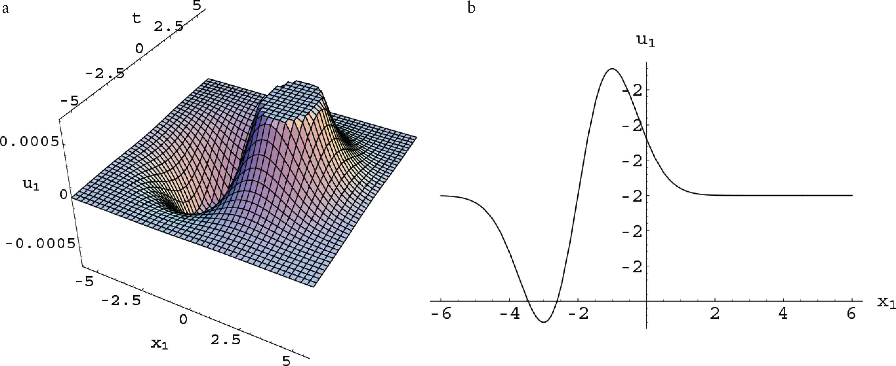
Plots for u1 in the solution (4.9). (a) Perspective view of the wave. (b) The propagation along x1 direction.
4.2. The Multiple Fusion Solutions
For constructing the multiple fusion solutions, we introduce the variable transformation via
One may readily verify that
Insertion of (4.12) into (3.4) produces a travelling wave solution to the NDB equation (1.4), which is in the form of
Interestingly, unlike the first type solution (4.8), such a solution (4.13) shows N-fusion phenomenon. For convenience, we take N = 2 as example to show the results, wherein the two-travelling wave solution to the (2 + 1)-dimensional Burgers system is given by
The 2-soliton fusion phenomenon of u1 can be clearly seen in Figure 2. From the pictures, we can see that there are two single kink-soliton collide and fusion to one at certain time. Such fusion phenomenon are very important, which have been observed in many physical models, like in organic membrane, macromolecule material, even-clump DNA, nuclear physics and Sr-Ba-Ni oxidation crystal (see [15,40,41]). Deep analysis shows that for all the ranges of the parameters a1j and a2j, only fusion can occur in the 2-solitons expressed by (4.14). Both elastic scattering and fission can not happen.
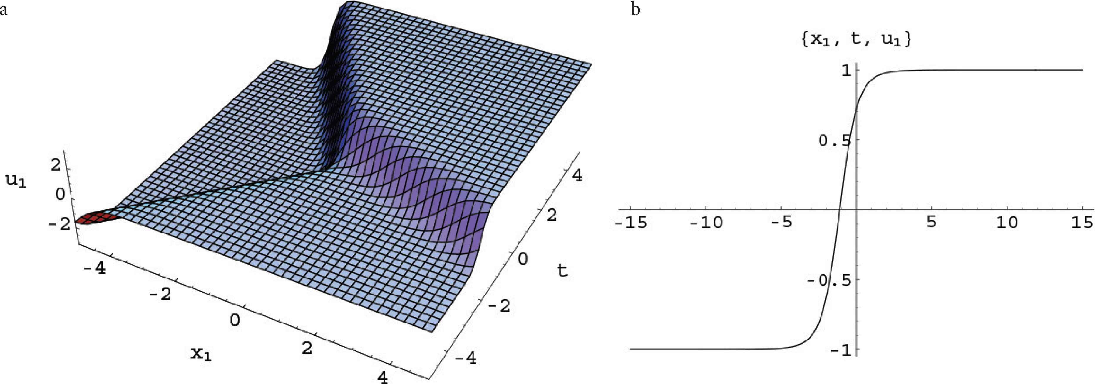
Plots of u1 in the solution (4.14). (a) Perspective view of the wave. (b) The propagation along x direction.
4.3. The Rational Solutions
Here, we aim to seek to the polynomial solution of heat equation (3.8) in the form of
Substituting (4.15) into (3.8) produces
So the solution of the heat equation (3.8) is
Inserting it into the Cole-Hopf transformation (3.4), the rational solution for the NDB system is obtained as follows
For t > 0 and x → ±∞, it shows that the solution uj tends to −2μcj.
For example, setting N = 1, the Burgers equation (1.1) admits a solution of
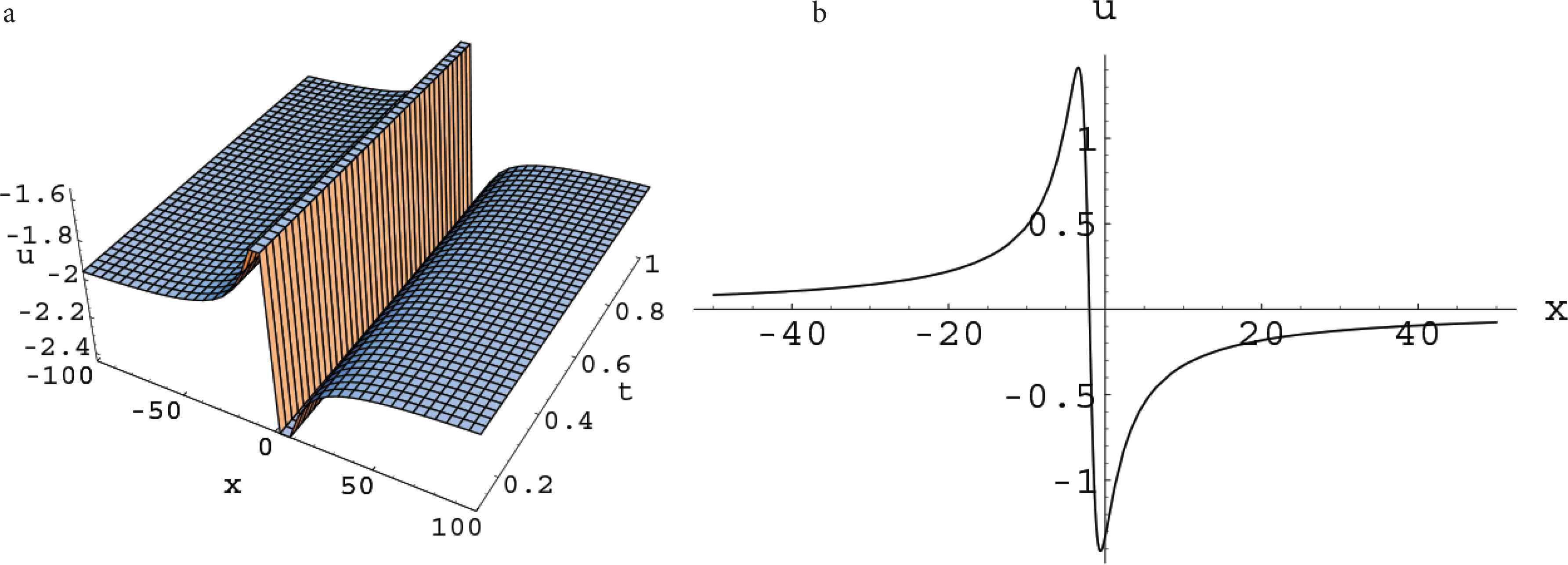
Plots of u in the solution (4.19). (a) Perspective view of the wave. (b) The propagation along x direction.
4.4. The Triangular Rational Solutions
Now, we search for a kind of triangular function solutions for the heat equation (3.8) in the form of
By substituting (4.20) into (3.8), we have
So the generalized heat equation (3.8) admits a solution
By using the Cole-Hopf transformation (3.4), we then find a kind of triangular rational solutions for NDB system
When N = 1, we get a triangular rational solution for the Burger equation (1.1)
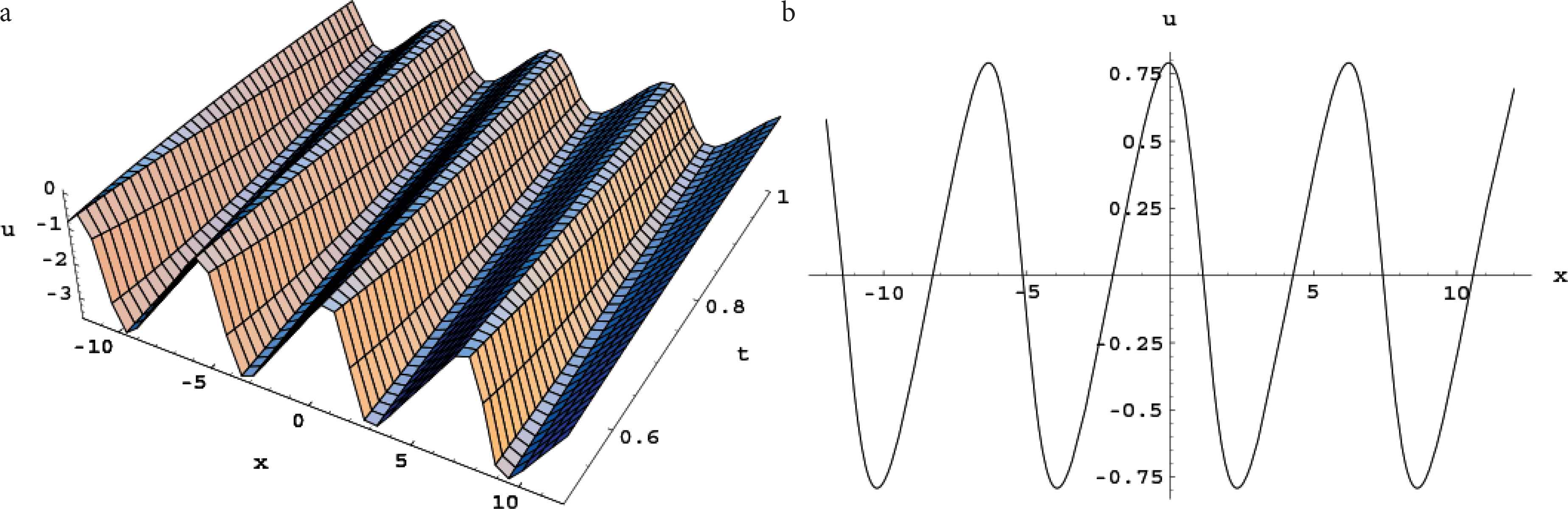
Plots of u in the solution (4.24). (a) Perspective view of the wave. (b) The propagation along x direction.
5. CONCLUSION
In this paper, the bilinear formulation for the (N + 1)-dimensional Burgers equation is established by using a fractal transformation. A special reduction of the bilinear formulation is introduced and thereby the generalized Cole-Hopf transformation is obtained, which leads to the general heat equation. When N = 1, the reduced general heat equation coincides with the some physical models (see Remarks 3.1 and 3.2). As applications of the N-dimensional Cole-Hopf transformation, some physically interesting solutions, such as vortex solutions, multiple fusion and two different types of rational solutions are given. Numerical analysis shows that these solutions exhibit physically interesting behaviors. However, there are some interesting problems that deserve further investigation. For example, since the momentum equation of the NDB system shares some similarities to that of the N-dimensional incompressible/compressible Euler equation and Navier–Stokes (NS) equation. Therefore, a natural question is that whether there exists appropriate bilinear formulations for the Euler and NS equations. If the answer is positive, then it means that we can quasi-linearize the Euler and NS equations. Based on the importance and wide applications of the two equations, these questions are worth deep investigations in the future.
CONFLICTS OF INTEREST
The authors declare they have no conflicts of interest.
ACKNOWLEDGMENTS
The authors would like to express their sincere thanks to the referees for their kind comments and valuable suggestions. This work is supported by the
REFERENCES
Cite this article
TY  - JOUR
AU  - Hongli An
AU  - Engui Fan
AU  - Manwai Yuen
PY  - 2020
DA  - 2020/12/10
TI  - The (N + 1)-Dimensional Burgers Equation: A Bilinear Extension, Vortex, Fusion and Rational Solutions
JO  - Journal of Nonlinear Mathematical Physics
SP  - 27
EP  - 37
VL  - 28
IS  - 1
SN  - 1776-0852
UR  - https://doi.org/10.2991/jnmp.k.200922.004
DO  - 10.2991/jnmp.k.200922.004
ID  - An2020
ER  -