
Symmetries, Conservation Laws, Invariant Solutions and Difference Schemes of the One-dimensional Green-Naghdi Equations
- DOI
- 10.2991/jnmp.k.200922.007How to use a DOI?
- Keywords
- Lie group; group classification; invariant solutions; conservation laws; invariant difference schemes
- Abstract
The paper is devoted to the Lie group properties of the one-dimensional Green-Naghdi equations describing the behavior of fluid flow over uneven bottom topography. The bottom topography is incorporated into the Green-Naghdi equations in two ways: in the classical Green-Naghdi form and in the approximated form of the same order. The study is performed in Lagrangian coordinates which allows one to find Lagrangians for the analyzed equations. Complete group classification of both cases of the Green-Naghdi equations with respect to the bottom topography is presented. Applying Noether’s theorem, the obtained Lagrangians and the group classification, conservation laws of the one-dimensional Green-Naghdi equations with uneven bottom topography are obtained. Difference schemes which preserve the symmetries of the original equations and the conservation laws are constructed. Analysis of the developed schemes is given. The schemes are tested numerically on the example of an exact traveling-wave solution.
- Copyright
- © 2020 The Authors. Published by Atlantis Press B.V.
- Open Access
- This is an open access article distributed under the CC BY-NC 4.0 license (http://creativecommons.org/licenses/by-nc/4.0/).
1. INTRODUCTION
An ideal fluid flows under the force of gravity can be modeled by means of the Euler equations. However, the full Euler equations are too complicated for describing waves on the surfaces of ideal fluid, in particular, because of free surface being a part of the solution. This difficulty motivated scientists for deriving simpler equations. One class of such equations is a class of shallow water equations. The classical approach of deriving the shallow water equations consists of approximation of the Euler equations for the irrotational flows. The hierarchy of the shallow water approximations is considered with respect to the shallowness parameter δ = h0/L, where h0 is the mean depth of the fluid, L is the typical length scale of the wave [29]1. In particular, the Green-Naghdi equations, derived for describing the two-dimensional fluid flow over an uneven bottom, are accurate to the dispersive terms of order δ2. The Green-Naghdi system of equations is the generalization of the equations derived first by Serre [39] and later by Su and Garden [42] to describe the one-dimensional propagation of fully nonlinear and weakly dispersive surface gravity waves over flat bottom. In the present paper we study the one-dimensional case of the Green-Naghdi equations.
Due to the significance of the Green-Naghdi model, there has been increasing interest in the numerical solving of the Green-Naghdi equations. The following numerical approaches have been developed for the Green-Naghdi system, based on either the finite difference, hybrid finite-difference finite-volume, pseudospectral and Galerkin/finite-element methods. Review of these methods can be found in [6, 16, 27, 33]. A numerical scheme developed in [17] is based on a different approach: the idea is to replace the dispersive Green-Naghdi equations by approximate hyperbolic equations. This approach was also applied in [18, 28].
In the present paper we use an approach based on the group properties of the Green-Naghdi equations. The group analysis method [34,35] yields exact solutions of differential equations, conservation laws via Noether’s theorem and a basis for invariant finite-difference schemes construction. Applications of group analysis to the Green-Naghdi equations with a horizontal bottom topography in Eulerian and Lagrangian coordinates were studied in [4, 40]. In particular, the authors of [40] applied Nother’s theorem for finding conservation laws of the Green-Naghdi equations. Notice that in order to apply the Noether theorem for finding conservation laws one needs to know an admitted Lie group. Another requirement is an existence of a Lagrangian providing that the underline equations are in the Euler-Lagrange form. This is one of the main advantages of the Lagrangian coordinates used in the present paper.
One of the main objectives of the present paper among the group classification and conservation laws is to construct a numerical scheme which inherits the group properties of the original equations. Earlier, in [13,14], this method was applied to the hyperbolic shallow water equations with an arbitrary bottom topography considered in Eulerian and Lagrangian coordinates. An invariant difference scheme possessing all difference analogues of the conservation laws was constructed there.
The one-dimensional Green-Naghdi equations describing surface gravity waves over uneven bottom have the form [5,19,24,30]
Assuming that
It should be noted here that for ε = 0 equations (1.1) become the hyperbolic shallow water equations. Symmetries, conservation laws and numerical schemes based on their group properties of the one-dimensional hyperbolic shallow water equations with different type of bottom topographies have been analyzed in Eulerian and Lagrangian coordinates in [1–4, 13–15, 23, 40].
In the present paper the one-dimensional equations (1.1) in mass Lagrangian coordinates (s, t) with the functions A and B of the form either (1.2) or (1.3) are studied. In [40], it is shown that the Green-Naghdi equations with horizontal plane bottom are equivalent to the Euler-Lagrange equation written in the mass Lagrangian coordinates. For the one-dimensional Green-Naghdi equations with uneven bottom there is the problem of finding a Lagrangian. If the Lagrangian is found, then one can apply Noether’s theorem for finding conservation laws.
Another objective of the present paper is to construct conservative numerical schemes which preserve both a symmetry of original differential equations and difference analogs of conservation laws.
The paper is organized as follows. Section 2 is devoted to the study of equations (1.1), (1.2) in Lagrangian coordinates: corresponding Lagrangians are found, and the group classification is carried out. Applying Noether’s theorem, conservation laws in Lagrangian and Eulerian coordinates are derived. Then, the similar study of equations (1.1), (1.3) is given in Section 3, where it is also shown that equations (1.1), (1.3) with a flat bottom topography Hb = qx + β are locally equivalent to the Green-Naghdi equations with a horizontal bottom topography Hb = const. Preliminary information essential for further construction of conservative finite-difference schemes is given in Section 4. A new three-layer invariant conservative finite-difference scheme for the Green-Naghdi equations with a horizontal flat bottom topography is constructed in Section 5. At the end of Section 5, the possibilities of extending the obtained difference scheme to the case of an arbitrary bottom profile are discussed. Application of the scheme for analysis of traveling wave type solutions of the Green-Naghdi equations are considered in Section 6. The results are summarized in Conclusion.
2. EQUATIONS (1.1), (1.2) IN LAGRANGIAN COORDINATES
2.1. Eulerian and Lagrangian Coordinates
Relations between Lagrangian Coordinates (t, ξ ) and Eulerian coordinates (t, x) for the one-dimensional case are defined by the condition x = φ(t, ξ), where the function φ(t, ξ ) is the solution of the Cauchy problem
In Lagrangian coordinates, the general solution of the mass conservation law equation is
Here the functions
Hence, the mass Lagrangian coordinates are defined by the equations
The corresponding equation becomes
2.2. Search for a Lagrangian
For finding a Lagrangian for which equation (2.3) is the Euler-Lagrange equation one has to solve the following problem. Let ℒ(t, s, φt, φs, φtt, φts, φss) be a corresponding Lagrangian. Then, substituting ℒ into the equation2
2.3. Group Analysis of Equation (2.3)
To find equivalence transformations we used the infinitesimal criterion [35]. For this purpose the determining equations for the components of generators of one-parameter groups of equivalence transformations were derived. The solution of these determining equations gives the general form of elements of the equivalence algebra of the class (2.3). The basis elements of the equivalence algebra of the class (2.3) are
In the group classification we use the transformations corresponding to the generators
It should be noted that the Galilean transformation corresponding to the generator
There are also the obvious involutions
Calculations show that the kernel of admitted Lie algebras is defined by the generators
An extension of the kernel only occurs for a linear bottom
Remark 2.1.
The same Lie group is admitted by the equations with the horizontal bottom (q = 0) studied in [40]. The coincidence of the admitted Lie groups proposes to assume that the Green-Naghdi equations with a flat bottom topography (2.4) are equivalent to the Green-Naghdi equations with a horizontal bottom q = 0. We have checked that if such a transformation exists, then it is not among the point transformations of the form
We have also checked that it is not among the point transformations of the form
2.4. Conservation Laws
A conservation law of equations either (1.1), (1.2) or (1.1), (1.3) in Lagrangian coordinates is considered in the following local form
Its counterpart in Eulerian coordinates has the form
Notice that if a generator X = ξt∂t + ξs∂s + ζ∂φ is either variational or divergently variational, then there exist such functions Bt and Bs that [21]
Hence, for either variational or divergently variational generator X, one has that
2.4.1. Conservation laws corresponding to the kernel of admitted Lie algebras
Conservation laws are obtained by applying Noether’s theorem.
The generator ∂s provides the conservation law with the densities:
In Eulerian coordinates the counterpart conservation law has the densities
The generator ∂t gives the conservation law of energy with the densities:
In Eulerian coordinates the densities of the corresponding conservation law are
2.4.2. Flat bottom topography
In this case one has that Hb = qx.
Using the general solution for a Lagrangian, it can be shown that the generator X = t∂t + 4s∂s + 2φ∂φ does not satisfy the condition (2.6).
The generator t∂φ corresponding to the Galilean transformation provides the conservation law with the densities:
In Eulerian coordinates this conservation law gives a the center-of-mass law:
The generator ∂φ provides the conservation law with the densities:
3. EQUATIONS (1.1), (1.3) IN LAGRANGIAN COORDINATES
3.1. Lagrangian Coordinates
Similar analysis of equations (1.1), (1.2) gives that in mass Lagrangian coordinates equations (1.1), (1.3) are equivalent to the equation
Following the same method of finding a Lagrangian for equation (3.1) as in the previous section, we derived the general form of the Lagrangian. A particular form of the Lagrangian providing equation (3.1) as the Euler-Lagrange equation
3.2. Equivalence Transformations
3.2.1. Equivalence group
Calculations give that equivalence group is defined by the generators
As in the previous case there are also the obvious involutions
3.2.2. Flat bottom
Consider the topography
Because of the equivalence transformation corresponding to the generator
Remark 3.1.
The property of the reduction of the shallow water equations with a flat bottom topography to the equations with the horizontal flat bottom is known for the one-dimensional hyperbolic shallow water equations [10]. For the two-dimensional hyperbolic shallow water equations it is proven in [31].
3.3. Group Classification
The kernel of admitted Lie algebras is defined by the generators
Extensions of the kernel occur for
if
Remark 3.2.
Similar extensions of a kernel of admitted Lie groups occur for the one-dimensional hyperbolic shallow water equations with a parabolic bottom topography [13,14,23]. In the case of two-dimensional hyperbolic shallow equations with a constant Coriolis parameter such type of extensions also occur for a circular paraboloid [25,31]. In the paper of Chesnokov [8] it was noted that for a circular parabolic bottom the admitted Lie algebra found in [25] is isomorphic to the Lie algebra admitted by the classical shallow water equations with a horizontal bottom Hb = const and zero Coriolis parameter. In [8, 31] it is proven that two-dimensional hyperbolic shallow equations with a constant Coriolis parameter with a circular parabolic bottom topography are locally equivalent to the classical gas dynamics equations.
3.4. Conservation Laws
3.4.1. Kernel of admitted Lie algebras
The kernel of admitted Lie algebras ∂s and ∂t gives the conservation laws with the densities, respectively:
Counterparts of these conservation laws in Eulerian coordinates have the densities:
3.4.2. Parabolic bottom topography
Using the general solution for a Lagrangian, it can be shown that the generators eqt∂φ and e−qt∂φ corresponding to the case k = −q2/(2εg) do not satisfy the condition (2.6). The other two generators sin(qt)∂φ and cos(qt)∂φ corresponding to the case k = q2/(2εg) provide the conservation laws, respectively:
In Eulerian coordinates the counterparts of these conservation laws contain the variable s, which satisfy the equations
These conservation laws have the densities:
4. PRELIMINARY ANALYSIS OF THE GREEN-NAGHDI EQUATIONS FOR CONSTRUCTING FINITE-DIFFERENCE SCHEMES
4.1. Conservative Form of the Equations in Lagrangian Variables
Before construction of finite-difference schemes we rewrite the Green-Naghdi equations for a horizontal bottom topography
The local conservation laws of momentum, energy, and center-of-mass law can be rewritten as follows
The conservation law of mass automatically follows from the symmetry of second derivatives xts = xst.
4.2. The Green-Naghdi Equations in Hydrodynamic Variables
Here we represent the Green-Naghdi equations in hydrodynamic variables u(t, s), ρ(t, s), where ρ3 is the depth of the fluid over the bottom and s, as before, is the mass Lagrangian coordinate.
It turns out to be especially convenient to use hydrodynamic variables in finite-difference space [13]. This allows transition from a three-layer finite-difference schemes to a two-layer ones.
The shallow water equations in hydrodynamic variables are obtained by the change
The Green-Naghdi equations become
The variable p(t, s) which was introduced in [36] by the relation
The local conservation laws of momentum (4.3), energy (4.5), and center-of-mass law (4.4) become
5. INVARIANT DIFFERENCE SCHEMES
5.1. Invariant Conservative Scheme
For constructing difference scheme one needs 9-nods stencil (see Figure 1), which has three-layers in time
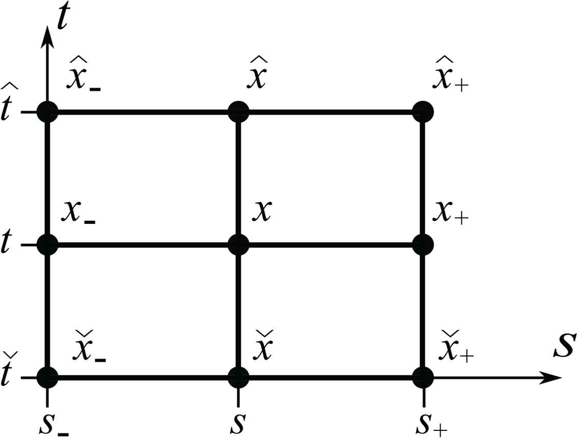
9-point stencil.
Here n- and m-indices correspond to the time and space layers appropriately, and the point (n, m) is fixed. For the sake of brevity we also use the following notation [38]
Here and further the simplest orthogonal regular mesh is considered
Indices of finite-difference variables are shifted by the finite-difference shift operators
The finite-difference total differentiation operators are defined through the shifts as
Notice that the operators
On the 9-nods stencil there was constructed invariant scheme for shallow water equations in [13]:
Analysis of the scheme along with consideration of difference invariants (5.8) suggests the following invariant extension for equation (5.4)
The scheme can also be obtained with the help of the finite-difference analog of so-called the ‘direct method’ (see [9,13,14] for discussion in detail).
Scheme (5.5) approximates equation (4.2) to the order O(τ2 + h2). It possesses the following local difference conservation laws:
- 1.
Conservation law of mass:
It automatically follows from the commutativity of the finite-difference differentiation on a uniform orthogonal mesh;
- 2.
Conservation law of momentum:
- 3.
Center-of-mass law:
- 4.
Conservation law of energy:
5.2. Invariant Representation of Scheme (5.5)
Scheme (5.5) admits the same Lie algebra as its differential counterpart, i.e., the generators
In 15-dimensional space of the difference stencil (5.2), there are 15 – 5 = 10 difference invariants:
Using the difference invariants (5.8), scheme (5.5) can be represented as follows
Hence, the invariant scheme and mesh are constructed. They possess the difference analogs of all conservation laws.
Remark 5.1.
All the generators (5.7) preserve the mesh uniformness and orthogonality (see criterion in [12]). This requirement is necessary for constructing invariant difference schemes on uniform orthogonal meshes, and it is often satisfied for the hydrodynamics-type schemes in Lagrangian coordinates.
5.3. Scheme (5.5) in Hydrodynamic Variables
Here we introduce finite-difference hydrodynamic variables through the relations constructed in [13] for the shallow water difference scheme, namely
The latter relation is an implicit approximation of equation (4.9), which allows one to preserve difference conservation laws.
Relations (5.9) and (5.10) allow one to write the scheme (5.5) in hydrodynamic variables on two time layers, i.e., to obtain a two-level scheme. But at the same time the additional equations must be added to the scheme. Hence, scheme (5.5) becomes
The scheme is defined on 6-point stencil (see Figure 2). One can check that equations of the system approximate system (4.7), (4.10) to the order O(τ + h). Notice that the first equation of system (5.11) follows from the equality
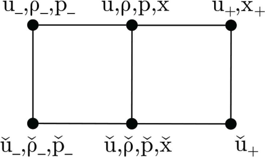
6-point stencil.
The conservation laws of scheme (5.11) are the following:
- 1.
The conservation of mass
- 2.
The conservation law of momentum:
- 3.
The center-of-mass law:
- 4.
The conservation law of energy:
5.4. On Extensions of the Scheme to the Case of Arbitrary Bottom
For model (1.1), (1.3) invariant scheme (5.5) can be extended to the case of an arbitrary bottom H(x) in the same manner as it was done in [13]. Indeed, adding
The construction of an invariant scheme that conserves both energy and momentum meets considerable difficulties. A separate example of invariant scheme that conserves momentum was proposed in [13] for the shallow water equations with an arbitrary bottom. It can be also generalized to the case of the Green-Naghdi equations.
6. TRAVELLING-WAVE TYPE SOLUTION FOR THE FINITE-DIFFERENCE SCHEME
6.1. Travelling-Wave Type Solution in Lagrangian Coordinates
To analyze some numerical properties of the constructed scheme, we consider Serre’s travelling-wave type solution [39] of the Green-Naghdi equations. In Eulerian coordinates, this type of solutions is invariant with respect to the generator ∂t and has the form4
In Lagrangian coordinates, the solution corresponds to the set of solutions invariant with respect to the generator ∂t + ∂s [40]. It has the following representation
The reduced equation (4.2) is
According to conservative form (4.2) of the equations, it can be rewritten as
Using the change
equation (6.3) becomes
If Θ = 0, then one gets the trivial solution
In case Θ ≠ 0 equation (6.4) has the first integral
In Eulerian coordinates it has the form
Notice that Serre’s solution satisfy the higher-order equation (6.3) only if R0 and A are related as follows
In order to perform computations in mass Lagrangian coordinates, one must find the initial distribution which correspond to solution (6.1). Hence, one must solve the Cauchy problem (2.1). For Serre’s solution it has the form
The solution for R0 = 0.75, γ = 1 is given in Figure 3 (left). The center of the soliton solution is shifted to the point xc = 50. The right side of Figure 3 demonstrates the numerical error of the transformations. The numerical solutions in Eulerian (6.7) and mass Lagrangian (6.8) coordinates for x ∈[0, 180] are given in Figure 4. The original analytical solution is not periodic and it is stable for small linear perturbations [26]. However, numerical calculations implement a periodic like solution (it was mentioned in [41]). Notice that this does not contradict the linear analysis since numerical calculations introduce finite perturbations. The quasiperiodicity of the numerical solution is confirmed by calculations with very small steps. Variation of steps from large to small does not affect the final solution sufficiently.

Relation for Eulerian and mass Lagrangian coordinates for Serre’s solution (R0 = 0.75, γ = 1). Left: the solution x(s) obtained numerically. Right: the numerical errors of the solution for |s(x(s)) – s| (solid line) and |x(s(x)) – x| (dotted line) confirm correctness of the relations between Eulerian coordinate x and mass Lagrangian coordinate s.

The Serre’s solution in Eulerian [41] (left) and mass Lagrangian (center and right) coordinates for R0 = 0.75 and γ = 1. The data for mass Lagrangian coordinates was obtained numerically. Solid line represents exact solutions corresponding to Serre’s solution (6.1). Dotted line represents numerical solutions obtained by Runge–Kutta methods.
6.2. Symmetry Reduction of the Scheme
Reduction of the invariant scheme on the subgroup ∂t + α∂s is the same as the reduction for the shallow water equations scheme [13]. The reduced scheme is
Equation (6.11) is a finite-difference analog of equation (6.3). To guarantee that new mesh spacing Δλ matches the original mesh nodes on the plane [12] (see Figure 5), one should assume that
Below h and τ are considered equal, which corresponds to α = 1.
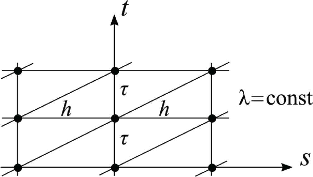
Relation between meshes in variables (s, t) and λ.
Remark 6.1.
It is worth mentioning that the difference shift operators in mass Lagrangian coordinates are related to the shift operators in λ-coordinates as follows
Changing the variables
If
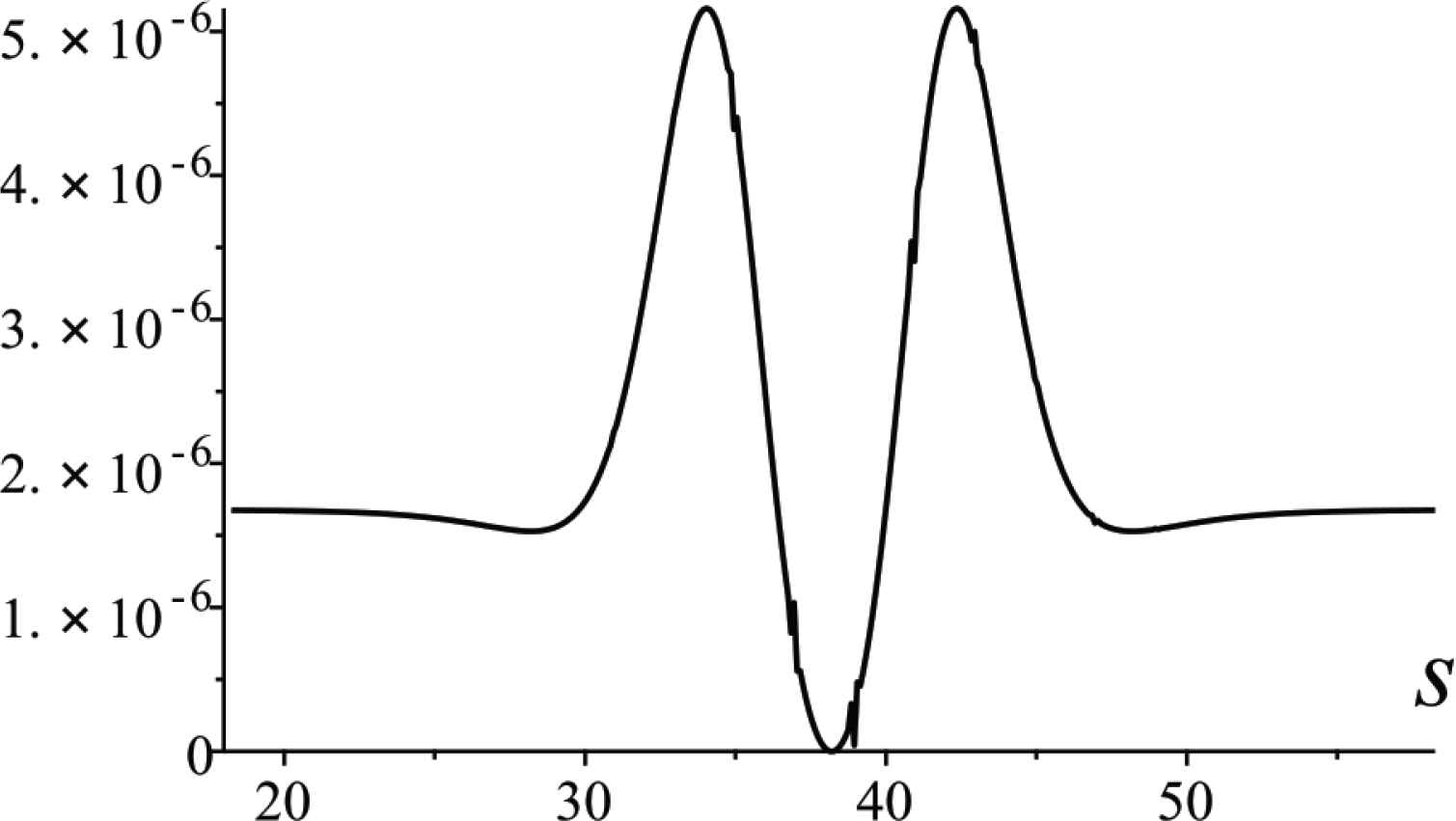
Preservation of the first integral (6.14) on the Serre’s solution.
The solution of the reduced scheme for the initial parameters, obtained by using Runge-Kutta method for equation (6.8), is presented in Figure 7. Notice that, as in the previous section, the numerical solution is periodic like.

Numerical solution of the reduced scheme (the initial data is given form the solution obtained by the Runge–Kutta type method). Solid line represents exact solution corresponding to Serre’s solution (6.1). Dotted line represents numerical solution of the reduced scheme.
6.3. Evolution of the Serre’s Solution for a Perturbed Scheme
Consider the second equation of scheme (5.11)
The term
In order to avoid these difficulties we consider the following perturbed version of equation (6.15)
This particular problem is also of independent interest. To clarify the physical meaning of this case, we refer to the paper [32], where it was considered a similar to (6.16) perturbed form of the Green-Naghdi equations in Eulerian coordinates. The perturbation coefficient α is responsible for the stability of the soliton solution. If its value tends to zero, the solution show dispersive qualities in time. In contrast to α, the value of the perturbation coefficient β does not essentially affect the profile of the free surface.
In particular, the evolution of the Serre’s solution for α = 0.001, β = 1, R0 = 0.75 and γ = 1 is presented in Figure 8. For the represented solution we explore a viscous version of the scheme, where the following change was used
Here v is a small viscosity coefficient. The dispersive wave forms are very similar to the results presented in [32] for small values of α.
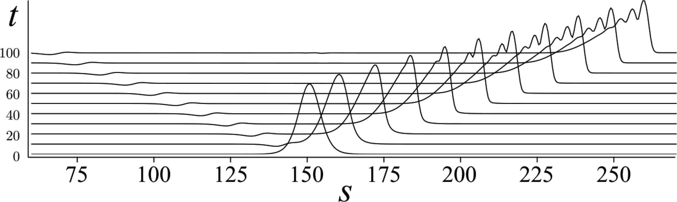
Evolution of the Serre’s solution for the perturbed scheme (6.16).
7. CONCLUSION
Group analysis of the one-dimensional Green-Naghdi equations describing the behavior of fluid flow over uneven bottom topography is given in the present paper. The Green-Naghdi equations are considered in two forms: in the classical form (1.1), (1.2) and in the mild slope approximation form (1.1), (1.3) which is of the same order as the original Green-Naghdi equations. Analysis of the studied equations is performed in Lagrangian coordinates. Working in the Lagrangian coordinates allowed us to find Lagrangians turning the analyzed equations into the Euler-Lagrange equations. It is shown that equations (1.1), (1.3) with a flat bottom topography Hb = qx + β are locally equivalent to the Green-Naghdi equations with a horizontal bottom topography Hb = const. Complete group classification of both cases of the Green-Naghdi equations with respect to the function Hb describing the uneven bottom topography is presented. Applying the Noether theorem, the developed Lagrangians and performed group classification, conservation laws of the one-dimensional Green-Naghdi equations with uneven bottom topography are obtained.
An invariant conservative finite-difference scheme is constructed for the Green-Naghdi equations for the case of a flat bottom topography. The scheme possesses the conservation laws of mass, momentum, energy and the center-of-mass law. This scheme is also represented in hydrodynamic variables. The representation in hydrodynamic variables simplifies its numerical implementation. The reduction of the invariant scheme on a subgroup is carried out similarly to the reduction of the corresponding differential equations. As a result of the reduction an ordinary finite-difference equation is obtained. This equation possesses a first integral, which is well preserved on Serre’s exact solution. Using the example of Serre’s solution further numerical analysis of the scheme is performed. The stationary solution, obtained by the proposed scheme, has the same qualitative properties as the solutions calculated by the Runge-Kutta methods. The time evolution of Serre’s solution is considered by the example of a specific perturbed version of the scheme which allows one to avoid working with large velocity gradients terms. The latter invariant scheme was generalized for an arbitrary bottom topography. This scheme also possesses the conservation laws of mass and energy.
CONFLICTS OF INTEREST
The authors declare they have no conflicts of interest.
ACKNOWLEDGEMENTS
The research was supported by
Footnotes
See also the references therein.
We use ρ instead of h, as h is usually accepted in numerical analysis for the finite-difference step.
Usually the independent variable in traveling waves has the form x − ct. Because of the Galilean transformation the constant c can be set to zero.
REFERENCES
Cite this article
TY  - JOUR
AU  - V.A. Dorodnitsyn
AU  - E.I. Kaptsov
AU  - S.V. Meleshko
PY  - 2020
DA  - 2020/12/10
TI  - Symmetries, Conservation Laws, Invariant Solutions and Difference Schemes of the One-dimensional Green-Naghdi Equations
JO  - Journal of Nonlinear Mathematical Physics
SP  - 90
EP  - 107
VL  - 28
IS  - 1
SN  - 1776-0852
UR  - https://doi.org/10.2991/jnmp.k.200922.007
DO  - 10.2991/jnmp.k.200922.007
ID  - Dorodnitsyn2020
ER  -