Journal of Nonlinear Mathematical Physics

Volume 27, Issue 4, September 2020, Pages 592 - 615

Asymptotics behavior for the integrable nonlinear Schrödinger equation with quartic terms: Cauchy problem

Authors
Lin Huang
School of Science, Hangzhou Dianzi University, Hangzhou 310018, P. R. China,lin.huang@hdu.edu.cn&linhuang@kth.se
Received 10 August 2019, Accepted 3 January 2020, Available Online 4 September 2020.
DOI
10.1080/14029251.2020.1819605How to use a DOI?
Keywords
Integrable nonlinear Schrödinger equation with quartic terms; Long-time asymptotics; Nonlinear steepest descent method
Abstract

We consider the Cauchy problem of integrable nonlinear Schrödinger equation with quartic terms on the line. The first part of the paper considers the Riemann-Hilbert formula via the unified method(also known as the Fokas method). The second part of the paper establishes asymptotic formulas for the solution of initial value problem using the nonlinear steepest descent method(also known as the Deift-Zhou method).

Copyright
© 2020 The Authors. Published by Atlantis Press and Taylor & Francis
Open Access
This is an open access article distributed under the CC BY-NC 4.0 license (http://creativecommons.org/licenses/by-nc/4.0/).

1. Introduction

The long-time asymptotics of initial value problem of integrable nonlinear evolution equations can be analyzed by means of the nonlinear steepest descent method introduced by Deift and Zhou [19]. In the context of initial value problems, the Riemann-Hilbert (RH) problem is formulated on the basis of certain spectral functions whose definitions involve the initial data of the solution [3, 40]. In this way, the long-time asymptotics for the solutions of decay initial value problem of the mKdV equation and the Schrödinger equation were analyzed respectively by Deift, Its and Zhou [17, 19]. This method developed by several authors [18, 27] and has already been used for:

  1. (a)

    For the integrable equation with 2 × 2 spectral problem (i.e., 2 × 2 Lax pair);

    1. (i)

      Decay initial value problem: modified KdV equation [19]; defocusing NLS(nonlinear Schrödinger equation) [17]; sine-Gordon equation [15]; Camassa-Holm equation [11]; modified NLS equation [29]; Fokas-Lenells equation [38]; Hirota equation [26]; short pulse equation [37];

    2. (ii)

      Nondecaying initial value problem: focusing NLS equation [8]; derivative NLS equation [39]; modified KdV equation [30]; Camassa-Holm equation [32];

    3. (iii)

      Decay initial boundary value problem: modified KdV equation [27]; derivative NLS equation [2], Hirota equation [23]; sine-Gordon equation [24];

    4. (iv)

      Time-periodic boundary value problem: focusing NLS equation [58], stimulated Raman scattering [33];

    5. (v)

      Nonzero boundary conditions at infinity: focusing NLS equation [4] focusing Kundu–Eckhaus equation [36].

  2. (b)

    For the integrable equation (system) with 3 × 3 spectral problem (i.e., 3 × 3 Lax pair);

    1. (i)

      Decay initial value problem: Degasperis-Procesi equation [10], coupled nonlinear Schrödinger equations [21]; Boussinesq equation [16]; Sasa-satsuma equation [22, 25, 28].

    2. (ii)

      Decay initial boundary value problem: Degasperis-Procesi equation [9].

The aim of this paper is to analyze long-time asymptotics for the initial value problem of the integrable nonlinear Schrödinger equation with quartic terms(NLSQ),

iqt+12qxx|q|2q+γ(qxxx6qx2q*4q|qx|28qxx|q|22qxx*q2+6q|q|4)=0,(1.1a)
theinitialdataq(x,0)=q0(x)𝒮()(1.1b)
where γ is positive constant and the 𝒮 (ℝ) is denote the Schwartz class on the line. This equation was first analysed by Lakshmanan, Porsezian, Danielin in papers [31, 34, 35], and it is a modified nonlinear Schrödinger equation that takes into account fourth order dispersion. The NLSQ equation was considered by many scientists, they obtained some especial solutions for the equation, for example, soliton solution [1,12], Breather solutions and rogue wave [13]. More recently, the quintic equation of the hierarchy has been considered in [14]. The authors show that a breather solution and get the locus of the eigenvalues in the complex plane which converts breathers into solitons. Considering the following Lax pair representation [1]:
ψx=Mψ,ψt=Nψ.(1.2)
where
ψ=(ψ1ψ2),(1.3)
M=iλσ3+(0iriq0)iλσ3+U,(1.4)
N=N4λ4+N3λ3+N2λ2+N1λ+N0
where
N4=(8iγ008iγ),N3=(08iγr8iγq),N2=i(1+4γqr4iγrx4iγqx14γqr)N1=i(2iγ(rxqqxr)r+4γqr2+2γrxxq+4γq2r+2γqxx2iγ(rxqqxr)),N0=(A1B1C1A1)A1=i(12qr3γq2r2γ(rxxqqxrx+qxxr))B1=12rx6iγqrrxiγrxxx,C1=i2qx+6iγqrqx+iγqxxx.

The zero-curvature equation reproduces the following equation,

iqt+12qxx+q2r+γ(qxxxx+6r2q3+4qrxqx+2q2rxx+6rqx2+8rqqxx)=0(1.5)

If we take r = − q*, then the equation (1.5) can be write as (1.1a).

Our main results are shown in Section 2. They state in the form of two theorems (Theorem 1–2). Theorem 2.1 is concerned with the construction of solutions of the initial value problem, and the proof relies on the RH techniques(also call Fokas method). Section 3 is devotes to Theorem 2.2. The proof is based on the nonlinear steepest descent approach of the Deift and Zhou [19].

2. Main results

The first theorem presents how to get the solutions of (1.1) can be constructed starting from the reflect coefficient function r(λ). Let 𝒮 (ℝ) denote the Schwartz class of smooth rapidly decaying functions.

Theorem 2.1

(Construction of solutions). Suppose r(λ) ∈ 𝒮 (ℝ). Define the 2 × 2-matrix valued jump matrix J(x, t, λ) by

J(λ)=(1|r(λ)|2r(λ)¯e2(iλx(8iγλ4iλ2)t)r(λ)e2(iλx(8iγλ4iλ2)t)1)(2.1)

Then the 2 × 2-matrix RH problem

  • M(x,t,λ) is analytic in λ ∈ ℂ \ ℝ.

  • The boundary value M±(x, t, λ) atsatisfy the jump condition

    M+(x,t,λ)=M(x,t,λ)J(x,t,λ),λ,

  • Behavior at

    M(x,t,λ)=𝕀+O(1λ),asλ.
    has a unique solution for each (x,t) ∈ ℝ2 and the limit limλ→∞(λ M(x,t,λ))12 exists for each (x,t) ∈ ℝ2. Moreover, the function q(x, t) defined by
    q(x,t)=2ilimλ(λM(x,t,λ))12(2.2)
    is a smooth function of (x,t) ∈ ℝ2 with rapid decay as |x| → ∞ which satisfies the integrable nonlinear Schrödinger equation with quartic terms (1.1) for (x, t) ∈ ℝ2.

Proof.

See Section 3.

The second theorem gives the long-time asymptotics of the solutions constructed in Theorem 2.1 in the sector 𝒫={(x,t)|(xt)2<127γ}.

Theorem 2.2.

Assuming 𝒫={(x,t)|(xt)2<127γ}, let q(x,t) be the solution of the Cauchy problem (1.1), then as t → ∞ and (x,t) ∈ 𝒫, we have

q(x,t)=18t(1+8γλ02)(((32λ02t(1+8γλ02))iv(λ0)/2eit(2λ02(4γλ02+1))eχ0(λ0))2(M1A)12)+18t(1+8γλ22)(((32λ22t(1+8γλ22))iv(λ2)/2eit(2λ22(4γλ22+1))eχ2(λ2))2(M1B)12)+12t(1+8γλ12)(((16λ12t(1+8γλ12))iv(λ1)/2eit(2λ12(4γλ12+1))eχ1(λ1))2(M1C)12)+O(logtt).(2.3)

In the region 0 < max{|λ0|, |λ1|, |λ2|} < M, M is a positive constant. Where λ0, λ1, λ2 are three stationary points of phase function which defined in (4.1). (M1A)12, (M1B)12, (M1C)12, ν(λ0), ν(λ1), ν(λ2) are defined by (4.32),(4.31), (4.33) and (4.6), respectively, χ0(λ0), χ1(λ1), χ2(λ2), are defined by following

χ0(λ0)=12πiλ1λ0ln(1|r(μ)|21|r(|λ0|)|2)dμμλ0χ2(λ2)=12πiλ1λ2ln(1|r(μ)|21|r(|λ2|)|2)dμμλ2χ1(λ1)=12πiiλ1±iiλ1ln(1|r(μ)|21|r(|λ1|)|2)dμμλ1.

Proof.

See Section 4

3. The proof of Theorem 2.1

In this part, we only give a sketch how to prove Theorem 2.1 from the inverse scattering transformation of NLSQ equation.

We extend the column vector ψ to a 2 × 2 matrix and letting

ψ=Ψe(iλx(8iγλ4iλ2)t)σ3,
then the Lax pair (1.2) can be rewritten as follows,
Ψxiλ[σ3,Ψ]=UΨ,(3.1a)
Ψt(8iγλ4iλ2)[σ3,Ψ]=VΨ(3.1b)
where U is defined by (1.4) and V is defined follows
V=N3λ3+(N2σ3)λ2+N1λ+N0(3.2)
which can be written in total differential form,
d(e[iλx+(8iγλ4iλ2)t)]σ^3Ψ(x,t,λ))=e[iλx+(8iγλ4iλ2)t]σ^3W(x,t,λ)Ψ,
where
W(x,t,λ)=Udx+Vdt=(0iq¯iq0)dx+(λU+12V+γVp)dt.

In order to formulate a RH problem for the solution of the inverse spectral problem, we seek solutions of the spectral problem which approach the 2 × 2 identity matrix as λ → ∞.

Throughout this section, assuming that q(x,t) is sufficiently smooth. Defining two solutions of (3.1a) and (3.1b) by

Ψj(x,t,λ)=𝕀+(xj,tj)(x,t)e[iλ(xx)(8iγλ4iλ2)(tt)]σ^3(Udx+Vdt),j=1,2,
where (x1,t1) = (−∞,t),(x2,t2) = (+∞,t).

This choice implies following,

Γ1:x>x,i.e.,xx>0,Γ2:x<x,i.e.,xx<0.

It means that we can write Ψj as:

Ψ1=𝕀+xeiλ(xx)σ^3U(x,t,λ)Ψ1(x,t,λ)dx,Ψ2=𝕀xeiλ(xx)σ^3U(x,t,λ)Ψ2(x,t,λ)dx.

It can be shown that the second column of Ψj is bounded and analytic in the following domain:

[Ψ1]2inlowhalfplane,[Ψ1]1inuphalfplane,[Ψ2]1inlowhalfplane,[Ψ2]2inuphalfplane.

According to the ordinary differential equation theory, it follows that the two solutions of (3.1) have linear relations,

Ψ1(x,t,λ)=Ψ2(x,t,λ)e[iλx(8iγλ4iλ2)t]σ^3S(λ),(3.3)
where
S(λ)=(s11(λ)s12(λ)s12(λ)s22(λ)).

It is easy to show that the following symmetry for Ψ(x,t,λ):

Ψ(x,t,λ)=σ1Ψ(x,t,λ¯)¯σ1,σ1(0110).

The symmetry implies as follows,

S(λ)=(a(λ)b(λ¯)¯b(λ)a(λ¯)¯).

Taking the sectionally meromorphic function M(x,t,λ) defined by

M(x,t,λ)={([Ψ1]1a(λ),[Ψ2]2),Imλ>0,([Ψ2]1,[Ψ1]2a(λ¯)¯),Imλ<0,
where [·]1 and [·]2 denote the first and second column, respectively.

By the analytic conditions of Ψ12,a(λ). It means that the function M(x, t, λ) is well-defined, and (3.3) can be rewritten as

M+(x,t,λ)=M(x,t,λ)J(λ),
where the jump matrix J(λ) is given by (2.1) with the function r(λ) = b(λ)/a(λ).

Remark 3.1.

Noticing that the jump matrix J(λ) in (2.1) is Hermite and positive. By the Zhou’ law [41], we can get the vanishing lemma for the Riemann-Hilbert problem M(x, t, λ). It means that the associated homogeneous RH problem has only the zero solution. In other wards, the solution of Riemann-Hilbert problem exists.

Substituting the asymptotic expansion

Ψ=D+Ψ1λ+Ψ2λ2+Ψ3λ3+O(1λ4),λ
into (3.1) and comparing the coefficients of λ, we find
O(λ):i[σ3,D]=0,(3.4)
O(1):Dx+i[σ3,Ψ1]=UD.(3.5)

Hence one can get D = 𝕀.

Inserting into the off-diagonal elements of (3.5), we can get

q(x,t)=2i(Ψ1)12,
that is,
q(x,t)=2ilimλ(λM(x,t,λ))12.
where M is the solution of the following RH problem: Given r(λ),λ ∈ ℝ, find a 2 × 2 matrix-value function M(x, t, λ) such that
  • M(x,t,λ) is analytic in λ ∈ ℂ \ ℝ.

  • The boundary value M±(x, t, λ) at Σ satisfy the jump condition

M+(x,t,λ)=M(x,t,λ)e(iλx(8iγλ4iλ2)t)σ^3J(x,t,λ),λ,(3.6)
where the jump matrix J(x, t, λ) is defined in terms of r(λ) by (2.1).
  • Behavior at ∞

    M(x,t,λ)=𝕀+O(1λ),asλ.

Lemma 3.1.

Define q(x, t) by (2.2), then

{Mx(x,t,λ)iλ[σ3,M(x,t,k)]=UM(x,t,λ),Mt(x,t,λ)+(8iγλ4iλ2)[σ3,M(x,t,k)]=VM(x,t,λ).(3.7)
where U and V are defined in terms of q(x, t) and the derivative of q(x, t) by (1.4) and (3.2), respectively.

Proof.

We can use the Foaks method and the dressing method to prove the lemma. The argument is analogous to that Lemma 4.1 in [25], so the proof will be omitted.

The compatibility condition of (3.7) shows that q(x, t) satisfies (1.1a). The proof of Theorem 2.1 is complete.

4. The proof of Theorem 2.2

In order to analyze the long-time behavior of the solution of the NLSQ equation, first we should split the jump matrix into an appropriate upper/lower triangular form which can help us to localize the problem to the neighborhood of the stationary point. An appropriate rescaling then reduces an oscillatory RH problem to a RH problem with constant coefficients, which can be solved explicitly in terms of classical functions.

4.1. The augmented RH problem

We begin with the decomposition of the complex λ-plane according to the signature of the real part of the phase of the conjugating exponential of the oscillatory RH problem, Re(2itθ(λ)), where

θ(λ)=xtλ+8γλ4λ2,(4.1)

Assuming x/t := ξ satisfies the inequality,

ξ2<127γ,
then the phase function θ (λ) have three real stationary points λ0 > λ1 > λ2. The signature table of Re(2itθ (λ)) is given in Figure 1.

Fig. 1.

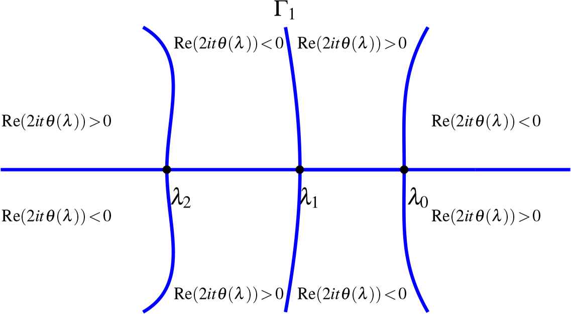
The signature of Re(2itθ (λ))

The main purpose of this section is to reformulate the original RH problem (Lemma 2.1) as an equivalent RH problem (see Lemma 4.1) on the augmented contour Σ (see Figure 2),

Fig. 2.

Augmented contour Σ.

=LL¯,
where,
L={λ;λ=λ0+λ0u2e3πi4,u(,2]}{λ;λ=λ2+|λ2|u2eiπ4,u(,2]}{λ;λ=λ1+|λ1|u2eiπ4,u(,2]}.(4.2)

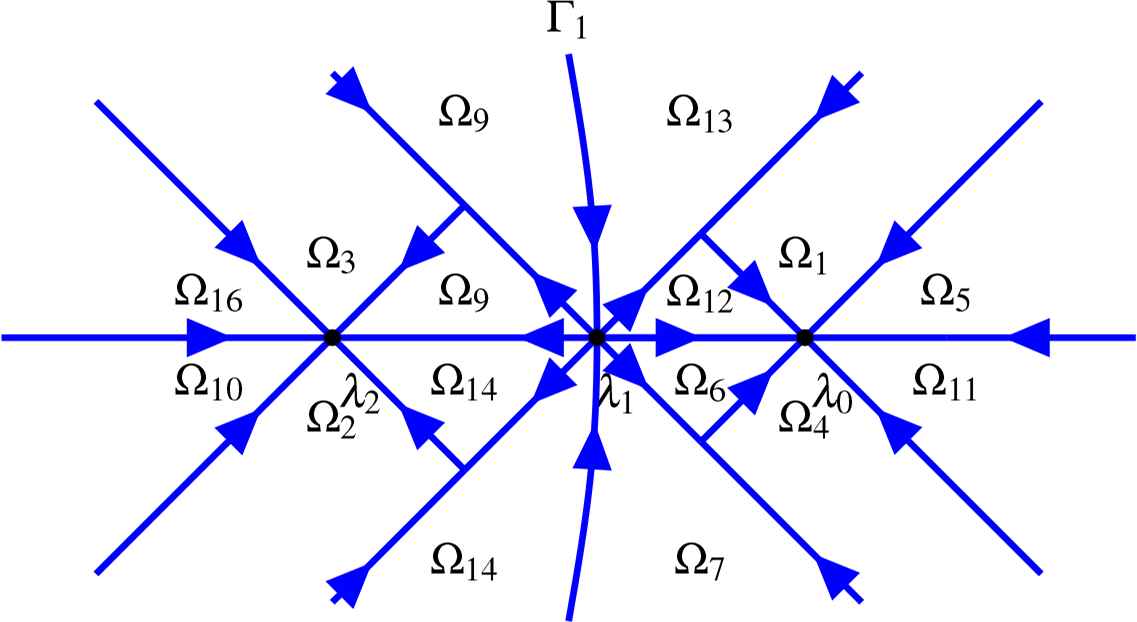
In order to define the conjugation matrices on Σ and exploit the analyses in [3, 19], we need to formulate two technical propositions: the first concerns the triangular factorisation of the conjugation matrices of the original RH problem (3.6), and the second pertains to a special decomposition for the reflection coefficient r(λ). The jump matrices (3.6) have following form,

eitθ(λ)σ3^G(λ)=eitθ(λ)σ3^(1r(λ)01)(10r(λ¯)¯1),
for λ ∈ (−∞,λ2) ∪ (λ0,+∞), and, the form
eitθ(λ)σ3^G(λ)=eitθ(λ)σ3^(10r(λ¯)¯(1r(λ¯)¯r(λ))11)×(1r(λ¯)¯r(λ)00(1r(λ¯)¯r(λ))1)(1r(λ)(1r(λ¯)¯r(λ))101).(4.3)
for λ ∈ (λ2,λ0) ∪ {(λ1i∞,λ + i∞) ∈ Γ1}.

In order to eliminate the diagonal matrix between the lower/upper triangular factors in (4.3), by the scheme in [19], introduce the function δ (λ) which solves the scalar RH problem:

δ+(λ)={δ(λ)=δ(λ),λ(,λ2)(λ0+),δ(λ)(1r(λ¯)¯r(λ)),λ(λ2,λ0){(λ1i,λ+i)Γ1}δ(λ)1asλ.(4.4)

According to the Plemelj formulae, it is straightforward to show that the solution of RH problem (4.4) is given by

δ(λ)=(λλ0λλ1)iν(λ0)(λλ2λλ1)iν(λ2)eχ+(λ)eχ(λ)eχ^+(λ)eχ^(λ),(4.5)
where
ν(λ0)=12πlog(1|r(λ0)|2),(4.6a)
ν(λ1)=12πlog(1|r(λ1)|2),(4.6b)
ν(λ2)=12πlog(1|r(λ2)|2),(4.6c)
and
χ+(λ)=12πiλ1λ0ln(1|r(μ)|21|r(λ0)|2)dμ(μλ),χ(λ)=12πiλ1λ2ln(1|r(μ)|21|r(λ0)|2)dμ(μλ),χ^+(λ)=λ1+iλ1ln(1r(μ¯)¯r(μ))(μλ)dμ2πi,χ^(λ)=λ1iλ1ln(1r(μ¯)¯r(μ))(μλ)dμ2πi

Proposition 4.1.

Let

f(z)={r(λ)¯1|r(λ)|2,λ(λ2,λ0){λ1i,λ+iΓ1},r(λ)¯,λ(,λ2)(λ0,).
Then f has a decomposition
f(λ)=hI(λ)+hII(λ)+R(λ),λ,
where R(λ) is piecewise rational and hII(λ) has an analytic continuation to L. Moreover, in the domain max{|λ2|,|λ1|,|λ0|} < M, the following estimates are valid as t → ∞,
|e2itθ(λ)hI(λ)|c(1+|λ|2)t,λ,|e2itθ(λ)hII(λ)|c(1+|λ|2)t,λL,|e2itθ(λ)R(λ)|Cec¯ɛ2,λLɛ,
where L is given by (4.2) and Lε is defined by follows
Lɛ={λ;λ=λ0+λ0u2e3πi4,u(ɛ,2]}{λ;λ=λ2+|λ2|u2eiπ4,u(ɛ,2]},{λ;λ=λ1+|λ1|u2eiπ4,u(ɛ,2]},

Then the conjugates

f(λ)¯=hI(λ)¯+hII(λ¯)¯+R(λ¯)¯
gives the same estimates for e2itθ(λ)hI(λ)¯, e2itθ(λ)hII(λ)¯ and e2itθ(λ)R(λ¯)¯ on L¯.

Proof.

The argument is analogously as in the proof of Proposition 1.92 in [19] by expanding ρ(λ) in terms of a rational polynomial approximation in the neighbourhood of the real, first-order stationary phase points, λ0, λ1, λ2.

Lemma 4.1.

Let m(x, t; λ) be the solution of the RH problem formulated in (3.6). Set mΔ(x, t; λ) ≡ m(x,t;λ)(Δ(λ))−1, where

Δ(λ)(δ(λ))σ3,
and δ (λ) is given by (4.5). Define
m(x,t;λ){mΔ(x,t;λ),λΩ1Ω2Ω3Ω4,mΔ(x,t;λ)(I(wa)x,t,δ)1,λΩ5Ω6Ω7Ω8Ω9Ω10,mΔ(x,t;λ)(I(w+a)x,t,δ)1,λΩ11Ω12Ω13Ω14Ω15Ω16.

Then m(x, t; λ) solves the following (augmented) RH problem on Σ,

m+(x,t;λ)=m(x,t;λ)vx,t,δ(λ),λ,m(x,t;λ)Iasλ,(4.7)
where
vx,t,δ(λ)(I(w)x,t,δ)1(I+(w+)x,t,δ)={(I(w0)x,t,δ)1(I+(w+0)x,t,δ),λ,(I(w+a)x,t,δ),λL,(I(wa)x,t,δ)1,λL¯,
and
(w±(0,a))x,t,δ=(δ±(λ))σ3^exp{itθ(λ)σ3^}w±(0,a),w±0=(0hI(λ)00),w+a=(0(hII(λ)+R(λ)00),w0=(00hI(λ)¯0),wa=(00(hII(λ¯)¯+R(λ¯)¯0)

Proof.

In terms of the function mΔ(x, t; λ) defined in the Lemma, the original oscillatory RH problem (3.6) can be rewritten in the following form,

m+Δ(x,t;λ)=mΔ(x,t;λ)(I(w)x,t,δ)1(I+(w+)x,t,δ),λ,mΔ(x,t;λ)Iasλ,
where
(w±)x,t,δ=(δ±(λ))σ3^exp{itθ(λ)σ3^}w±,
and
w+=(0ρ(λ)00),w=(00ρ(λ¯)¯0).

Then the new RH problem is equivalent to the RH problem (3.6).

4.2. RH Problem on the Truncated Contour

In this section we show how to convert the RH problem (4.7) on Σ to a RH problem on a truncated contour with controlled error terms.

From the above section we have

q˜(x,t)=2ilimλ(zmΔ(x,t,λ))12=ilimλλ([σ3,mΔ(x,t,z)])12=ilimλλ([σ3,m(x,t,z)])12.
We can take the limit z → ∞ in Ω1, where mΔ(x, t, z) = m(x, t, z), so
q˜(x,t)=ilimλλ([σ3,m(x,t,λ)])12.(4.8)

The RH problem (4.7) can be solved as follows (see, for example, [3]). Let

(C±f)(λ)=f(ζ)ζλ±dζ2πi,λ,fL2(),(4.9)
denote the Cauchy operator on Σ oriented as in Figure 2.

Thus, for example, for λ > λ0 we have (C+f)(λ)=limɛ0f(ζ)ζ(λiɛ)dζ2πi, etc. As is well known, the operators C± are bounded from L2(Σ) to L2(Σ), and C+C = 1. Also, by scaling, we know that the bounds on C± : L2(Σ) → L2(Σ) are independent of the stationary points.

Define

Cwx,t,δ1f=C+(f(w1)x,t,δ)+C(f(w+1)x,t,δ),(4.10)
for 2×2 matrix-valued functions f. By Proposition 4.1, Cwx,t,δ1 is a bounded map from L2(Σ)+L(Σ) into L2(Σ). Let μ1′ = μ1′(z; x, t) ∈ L2(Σ) + L(Σ) be the solution of the basic inverse equation
μ1=𝕀+Cwx,t,δ1μ1.(4.11)

By the method of Beals and Coifman,

m(x,t,λ)=𝕀+μ1(ζ;x,t)wx,t,δ1(ζ)ζλdζ2πi,λ\(4.12)
is the unique solution of the RH problem (4.7). Indeed,
μ±1=𝕀+C±(μ1wx,t,δ1)=μ1(b±1)x,t,δ

Substituting formula (4.12) into (4.8), we learn that

q(x,t)=(1[σ3,μ1(ζx,t)wx,t,δ1(ζ)]δζ2πi)12=(1[σ3,((𝕀Cwx,t,δ1)1)(ζ)wx,t,δ1(ζ)]δζ2πi)12.

Let we : Σ → M(2, ℂ) be a sum of three terms

we=wa+wb+wc.(4.13)
we then have the following:
{wa=wx,t,δ1|issupportedonandiscomposedoftermsoftypehIandhI¯.wbissupportedonLL¯andiscomposedofthecontributiontowx,t,δ1fromtermsoftypehIIandh¯I.wcissupportedonLɛL¯ɛandiscomposedofthecontributiontowx,t,δ1fromtermsoftypeRandR¯.

Set

=\(LɛL¯ɛ)
with the orientation as in Figure. 3. Define w′ through
wx,t,δ1=w+we.

Fig. 3.

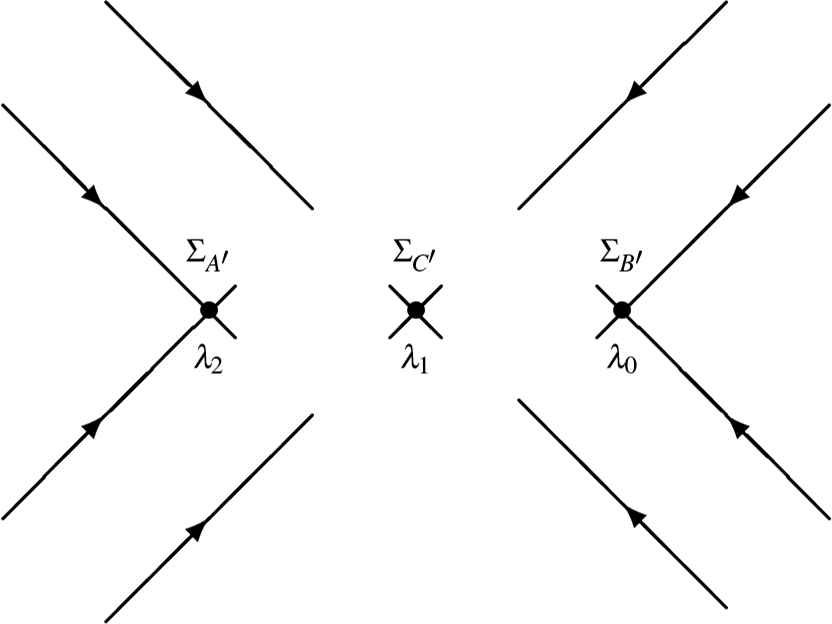
Truncated contour Σ′.

Observe that w′ = 0 on Σ\Σ′.

Lemma 4.2.

For arbitrary l ∈ 𝕑⩾1 and sufficiently small ε ∈ ℝ>0, as t → +∞ such that λ′ = min{|λ0|,|λ1|,|λ2|}>M,

wak(2×2)()c(λ2t)l,wbk(2×2)(LL¯)c(λ2t)l,wck(2×2)(Lδ^Lɛ¯)c_e2λ4ɛ2t,w2(2×2)()c(λ2t)1/4,w1(2×2)()c(λ2t),
where k ∈{1, 2, ∞}.

Proof.

By the conclusion of Proposition 4.1, the following estimates,

(w±)x,t,δ,wx,t,δk(2×2)()(2×2)(),k{1,2},
and analogous calculations as in Lemma 2.13 of [19]

Definition 4.1.

Denote by 𝒩 (·) the space of bounded linear operators acting in 2(2×2)().

Lemma 4.3.

As t →+∞ such that λ0 > M,(Id_Cwx,t,δ)1𝒩()(Id_Cw)1𝒩().

Proof.

Using the consequence of the following inequality, Cwx,t,δCw𝒩()c_we(2×2)(), the fact that we(2×2)()(c_|x|l)c_(λ2t)lc_ ((4.13) and Lemma 4.2), and the second resolvent identity.

Proposition 4.2.

If (IdCw)−1𝒩 (Σ), then for arbitrary l ∈𝕑⩾1, as t → + ∞ such that λ0 >M,

q(x,t)=i([σ3,((Id_Cw)1I)(ξ)]dξ2πi)21+𝒪(ctl).

Proof.

Using second resolvent identity and analogous calculations as (2.27) and Proposition 2.63 in [19] (or, Proposition 5.1 in [29], Proposition 3.19 in [26])

In the sense of appropriately defined operator norms, let us show that it may always choose to minus (or plus) a part of contour on which the jump matrix is I+𝒪(c_(λ02t)l), l ∈ 𝕑⩾1 and arbitrarily large, and without altering the RH problem,

Let:

  • R ∑′: 2(2×2)()2(2×2)() denote the restriction map;

  • I_:2(2×2)()2(2×2)()denote the embedding;

  • Cw:2(2×2)()2(2×2)() denote the operator in (4.10) with ww′;

  • Cw:2(2×2)()2(2×2)() denote the operator in (4.10) with ww′|Σ′ ;

  • CwE:2(2×2)()2(2×2)() denote the restriction of CwE to 2(2×2)();

  • IdΣ′ and IdΣ denote, respectively, the identity operators on 2(2×2)() and 2(2×2)().

Lemma 4.4.

CwCwE=CwECw,(Id_Cw)1=R(Id_Cw)1I_,(Id_Cw)1=Id_+CwE(Id_Cw)1R.(4.14)

Proof.

See Lemma 2.56 in [19].

Proposition 4.3.

If (Id_Cw)𝒩(), then for arbitrary l ∈𝕑⩾1, as t →+∞ such that λ0 >M,

q(x,t)=i([σ3,((Id_Cw)1I)(ξ)w(ξ)]dξ2πi)21+𝒪(ct).(4.15)

Proof.

The boundedness of (Id_Cw)1𝒩() follows from the assertion of the Lemma and (4.14) : the remainder is a consequence of Proposition 4.2.

From Proposition 4.3 we obtain that the asymptotic behavior can be constructed by the following RH problem on the contour Σ′,

m+(x,t;λ)=m(x,t;λ)vx,t,δ(λ),λ,m(x,t;λ)Iasλ,λ\,(4.16)
where vx,t,δ(λ)=(I(w)x,t,δ)1(I+(w+)x,t,δ), with
(w+)x,t,δ=(δ(λ)))σ3^eitθ(λ)σ3^R(λ)(0100),(w)x,t,δ=0,λL\Lɛ,(w+)x,t,δ=0,(w)x,t,δ=(δ(λ))σ3^eitθ(λ)σ3^R(λ)¯(0010),λL¯\Lɛ¯.

Denote (w)x,t,δ=(w+)x,t,δ+(w)x,t,δ, so that (w)x,t,δ=w| ; then, using the Beals-Coifman theory, the solution of RH problem (4.16) is shown as follows,

m(x,t;λ)=I+μ(x,t;ξ)(w(ξ))x,t,δ(ξλ)dξ2πi,λ\,
where μ(x,t;λ)(Id_Cw)1I.

4.3. RH Problem on the Disjoint Crosses

In this section, we will show that how to separate out the contributions of the three crosses in Σ′ to the solution q(x,t) in the formula (4.15). The main result in this part is Proposition 4.5.

Let us introduce some notations which for exact formulations. Taking Σ′ as the disjoint union of the three crosses, ΣA′, ΣB′, and ΣC′, extend the contours ΣA′, ΣB′, and ΣC′ (with orientations unchanged) to the follows,

^A={λ;λ=λ2+|λ2|u2e±iπ4,u},^B={λ;λ=λ0+λ0u2e±3πi4,u},^C={λ;λ=λ1+|λ1|u2e±iπ4,u},
and define by ΣA, ΣB, and ΣC, respectively, the contours {λ;λ=λ1+|λ1p|u2e±iπ4,u} oriented inward as in ΣA′ and ^A, inward as in ΣB′ and ^B, and inward/outward as in ΣC′ and ^C.

Let us prepare the following operators, for k ∈ {A,B,C},

Nk:2(^k)2(k),f(λ)(Nkf)(λ)=f(λk+ɛk),
where
λA=λ2,λB=λ0,λC=λ1,ɛ=λ(8t(1+8γλ2))1/2,=A,B,C.
Taking action of the operators Nk on function δ (λ)eitθ(λ), it find that, for k ∈ {A,B,C}, IA ≡ (−∞,λA), IB (λB,+∞), and IC ≡ (λA,λB),
Nk{δ(λ)eitθ(λ)}=δk0δk1(λ),Re(λ)Ik,
where,
δA0=(8tλ22(1+8γλ22))iv2exp{2iλ22(1+8γλ22)t+mχm(λk)},(4.17)
δB0=(8tλ02(1+8γλ02))iv2exp{2iλ02(1+8γλ02)t+mχm(λk)},(4.18)
δC0=exp{mχm(λ1)},(4.19)
δB1(λ)=(λλ0)iv(ɛB+2λB)iv(ɛB+λB)2ivexp{iλ22(1+ɛB2λ0)2+m(χm(λB+ɛB)χm(λB))},
δA1(λ)=(λλ2)iv(ɛA+2λA)iv(ɛA+λA)2ivexp{iλ22(1+ɛA2λ2)2+m(χm(λA+ɛA)χm(λA))},
δC1(λ)=((ɛCλ0)(ɛCλ2))ivexp{iλ22(1+2ɛCλ2)(12ɛCλ0)+m(χm(ɛC)χm(λ1))},
with ≡ {A,B,+,−}, and
χk(λ)=12πiλCλkln(1|r(μ)|21|r(|λ|)|2dμ(μλ))
χ±(λ)=i2πλ±λCln|iμλl|dln(1|r(iμ)|2),
χk(λC)=i2πλCλkln|μ|dln(1|r(μ)|2),
χ±(λC)=iλC+iiλCln(1+|r(μ)|2)μdμ2πi.

Set

Δk0=(δk0)σ3,
and let Δk0˜ denote right multiplication by Δk0:
Δk0˜ϕϕΔk0.

Denote

wk(λ)={(w)x,t,δ,λk,0,λ\k,andw^k(λ)={wk,λk,0,λ^k\k.

Then we have,

(w)x,t,δ=k{A,B,C}wk,C(w)x,t,δCw=k{A,B,C}Cwkk{A,B,C}Cwk.

In the remainder of this section, we remove the special notation for wk|k. We first show that some technical results concerning the operators Cwkk and Cw^k^k.

Proposition 4.4.

For k ∈ {A,B,C},

Cw^k^k=(Nk)1(Δk0˜)1Cwkk(Δk0˜)Nk,wk(Δk0)1(Nkw^k)(Δk0),
where
Cwkk|2(2×2)(Lk¯)=C+(.(R(ɛk+λk)¯(δk1(λ))2σ)),Cwkk|2(2×2)(Lk)=C(.(R(ɛk+λk)¯(δk1(λ))2σ+)).

The contours Lk are defined following,

Ll={λ;λ=λu2(8t(1+8γλ2))1/2eiπ4,u(ɛ,+)},{A,B},LC{λ;λ=|λ1|u2(8t(1+8γλ12)1/2eiπ4,u},
it means that k=LkLk¯.

Proof.

Analogous to the prove of Lemma 3.5 in [19], Proposition 6.1 in [29] or Lemma 3.20 in [26].

We introduce following expressions

R(λj+)limReλ>λjR(z)=r¯(λj);R(λj)limReλ<λjR(z)=r¯(λj)(1|r(λj)|2).

Lemma 4.5.

Let κ ∈(0,1). Then λLk¯k, as t →+∞ such that λ0 > M,

|R(ɛk+λk)¯(δk1(λ))2R(λk±)¯(λ)2iνeisgn(k)λ2|C(λk)|eiγ/2λ2|(1(tλ22(1+8γλk2))1/2+log(t|c(λ0,λ1,λ2)|)(t|λk|)1/2)
andλLk ⊂ Σk,
|R(ɛk+λk)(δk1(λ))2R(λk±)(λ)2iνeisgn(k)λ2|C(λk)|eiγ/2λ2|(1(tλk2(1+8γλk2))1/2+log(t|c(λ0,λ1,λ2)|)(t|λk|)1/2)
where Lk (resp. Lk¯), k ∈ {A,B,C}, are defined in Proposition 6.1, u ∈ (−ε,+∞), with 0<ɛ<2.

Proof.

Analogous of Lemma 3.35 in [19] (or Lemma 6.1 in [29]).

Lemma 4.6.

([29]). For general operators Cwk, k ∈ {1,2,…,N}, if (Id_Cwk)1 exist, then

(Id_+1αNCwα(Id_Cwα)1(Id_1βNCwβ)=Id_1αN1βN(1δαβ)(Id_Cwα)1CwαCwB,
and
(Id_+1βNCwβ(Id_+1αNCwα(Id_Cwα)1)=Id_1αN1βN(1δαβ)CwαCwβ(Id_Cwβ)1,
where δαβ is the Kronecker delta.

Lemma 4.7.

For αβ ∈ {A′,B′,C′}, as t → +∞ such that λ0 >M,

CwαCwβ𝒩()c_λ0t,CwαCwβ(2×2)()2(2×2)()c_(λ02t)1/4λ04t.

Proof.

Analogous to Lemma 3.5 in [19].

Proposition 4.5.

If, for k ∈ {A,B,C}, (Id_kCwk)1𝒩(k), then as t →+∞ such that λ0 >M,

P(x,t)=ik{A,B,C}(k[σ3,((Id_kCwkk)1I)(ξ)wk(ξ)]dξ2πi)21+𝒪(C(λ0,λ1,λ2)c_t).(4.20)

Proof.

Analogous of (2.27) in [19] and the second resolvent identity, one writes

(Id_k{A,B,C}Cwk)1=D_+D_(Id_E_)1E_,(4.21)
where
D_Id_+k{A,B,c}Cwk(Id_Cwk)1,E_α,β{A,B,C}(1δαβ)CwαCwβ(Id_Cwβ)1.

From the Lemma 4.2,

Cwk𝒩()wk2(2×2)()c_(λ02t)1/4c_,
and, take assumption (Id_Cwk)1𝒩()<, by means of Lemma 4.7, it is show that, as t → +∞ then,
D_𝒩()c_,and(Id_E_)1𝒩()c_,
as λ0 >M. Taking account of the second resolvent identity, it is simple to show that,
E_I2(2×2)()α,β{A,B,C}(1δaβ)CwαCwβI2(2×2)()+α,β{A,B,C}(1δaβ)CwαCwβ𝒩()(Id_Cwβ)1𝒩()CwβI2(2×2)().

According to Lemma 4.2,

CwkI2(2×2)()wk2(2×2)()c_(1+8γλ02t)1/4,
by the Lemma 4.7 and the second resolvent identity,
E_I2(2×2)()c_(1+8γλ02)t3/4.

According to the Cauchy-Schwarz inequality and Lemma 4.2,

E_w1(2×2)()E_I2(2×2)()w2(2×2)()c_(1+8γλ02)t;
hence, recalling (4.21), (Id_k{A,B,C}Cwk)1𝒩(). From Proposition 4.2 and the above estimates such that,
((Id_Cw)1(ξ)w(ξ)dξ=(D_I)w(ξ)dξ+𝒪(c_(1+8γλ02)t)+𝒪(c_((1+8γλ02)t)l)(4.22)
as t → +∞, for λ0 > M and arbitrary l ∈ 𝕑⩾1. Recall that w=k{A,B,C}wk, the integral on the right-hand side of (4.22) can be written following:
(D_I)w(ξ)dξ=(Id_k{A,B,C}wk+α,β{A,B,C}Cwαk((Id_Cwα)1I)wβ)(ξ)dξ.(4.23)

By Lemma 4.7 and the assumption that (Id_Cwk)1𝒩()<. Applying the second resolvent identity to the right-hand side of (4.23), it is show that,

((Id_Cw)1I)(ξ)w(ξ)dξ=k{A,B,C}((Id_Cwk)1I)(ξ)wk(ξ)dξ+𝒪(c(λ0,λ1,λ2)c_t),(4.24)
for arbitrary l ∈𝕑⩾1. Now, from Lemma 4.4,
(Id_kCwkk)1=Rk(Id_Cwk)1I_k;(4.25)

Then, substituting identity (4.25) into (4.24), and recalling (4.21) and (4.22), the proof is complete.

Lemma 4.8.

For k ∈ {A,B,C},(Id_kCwk)1𝒩(k).

Remark 4.1.

The Lemma 4.8 was proved in [19, 29]: In order to obtain the explicit asymptotic formulae presented in Theorem 2.2. we need a model RH problem which arises in crosses.

Proof.

We only consider the case k=B, the cases k=A and C follow in an analogous manner. From Lemma 4.3, by the fact that the boundedness of (1^BCωB^B)1, it follows that the boundedness of (1BCωBB)1. We note that

(1^BCωB^B)1=(NB)1(ΔB0)˜1(1BCωBB)1(ΔB0)˜NB,(4.26)
and then the boundedness of (1^BCωB^B)1 follows from the boundedness of (1BCωBB)1.

Set

ωB=(ΔB0)1(NBω^B)ΔB0,
so that
CωBB=C+(ωB)+C(ω+B).

On ΣB, we have the diagram in Figure. 4(a)

Fig. 4.

(a) ΣB; (b) ΣB,r; and (c) Σex ≡ ΣB,r ∪ ℝ.
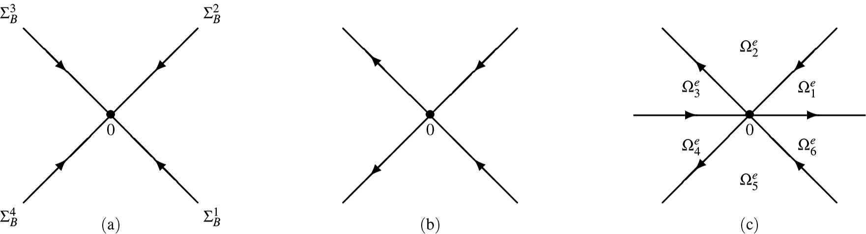
Set JB0=(bB0)1b+B0=(𝕀ωB0)1(𝕀ω+B0). Defining as usual ωB0=ω+B0+ωB0, and using Lemma 4.5, it is show that

ωBωB0L(BL1(B)L2(B)C(λ0)t12.(4.27)

Hence, as t → ∞,

CωBBCωB0BL2(B)C(λ1)t12,(4.28)
and consequently, one sees that the boundedness of (1BCωBB)1 follows from the boundedness of (1BCωB0B)1 as t → ∞.

Then reorient ΣB to ΣB,r as Figure. 4(b). A simple computation shows that the jump matrix JB,r=(bB,r)1(b+B,r)=(𝕀ωB,r)1(𝕀ω+B,r) on ΣB,r is determined by

ω±B,r(λ)=ωB0(λ),forReλ>0,
and
ω±B,r(λ)=ω±B0(λ),forReλ<0,

The third step is that extending ΣB,r Σe = ΣB,r ∪ ℝ with the orientation on ΣB,r as Figure. 4(c) and the orientation on ℝ from −∞ to ∞. And the jump Je=(be)1b+e=(𝕀ωe)1(𝕀ω+e) with

ωe(λ)=ωB,r(λ),λB,r,
ωe(λ)=0,λ.

Set Cωe on Σe. Once again, by Lemma 4.4, it is sufficient to bound (1ΣeCωe)−1 on L2e).

Then define a piecewise-analytic matrix function ϕ as follows:

M˜(λ0)=M(λ0)ϕ,
where
ϕ={λiνσ3,λΩ2e,Ω5e,λiνσ3(10r(λ0)eiλ221),λΩ1e,λiνσ3(1r(λ0)¯eiλ2201),λΩ6e,λiνσ3(1r(λ0)¯1|r(λ0)|2eiλ2201),λΩ3e,λiνσ3(10r(λ0)¯1|r(λ0)|2eiλ221),λΩ4e.

Thus, we can get the RH problem of M˜(λ0)

M˜+(λ0)(x,t,k)=M˜(λ0)(x,t,k)Je,ϕ,
M˜(λ0)(x,t,k)=(𝕀+M1B0λ+O(1λ2))λiνσ3,λ.
where
Je,ϕ={(1|r(λ0)|2r(λ0)¯eiλ22r(λ0)eiλ221),z𝕀,λB,r.

On ℝ we have

Je,φ=(be,φ)1b+e,φ=(𝕀ωe,φ)1(𝕀ω+e,φ)=(1eiλ22r¯(λ0)01)(10eiλ22r¯(λ0)1).
this completes the proof.

4.4. Model RH Problem

In this section, we will convert the evaluation of the integral in the Lemma 4.3 into three solvable RH problems on ℝ.

For j ∈ {A,B,C}, define

Mj(z)=𝕀+j((1jCωj0j)1𝕀)(ξ)ωj0(ξ)ξzdξ2πi,z\j.

Then, Mj(z) solves the RH problem

{M+j(z)=Ml(z)Jj(z)=Mj(z)(𝕀ωj0)1(𝕀+ω+j0),zj,Mj(z)𝕀,z.

If we take the asymptotic expansion,

Mj(z)=𝕀+M1jz+O(z2),z,
then
M1j=j((1jCωjj)1𝕀)(ξ)ωj(ξ)dξ2πi.(4.29)

Substituting into (4.20) of Proposition 4.5 and observe that inequalities (4.27) and (4.28) (and their analogues for ΣA and ΣC), we obtain

q(x,t)18t(1+8γλ02)(δB0)2(m1B)12+18t(1+8γλ22)(δA0)2(m1A)12+18t(1+8γλ12)(δC0)2(m1C)12+O(C(λ0,λ1,λ2)logtt).
where, the function C(λ0,λ1,λ2) is bounded in the sector 𝒫 defined in Theorem 2.2. i.e.,
q(x,t)18t(1+8γλ02)(δB0)2(m1B)12+18t(1+8γλ22)(δA0)2(m1A)12+18t(1+8γλ12)(δC0)2(m1C)12+O(logtt).(4.30)

Analogous of the references [19, 26, 29], when we consider the case B, write

Ψ=M˜(λ0)eiλ24σ3=Ψ^λiνσ3eiλ24σ3.

We have,

Ψ+(λ)=Ψ(λ)J˜(λ0),λ,
where
J(λ0)=(1|r(λ0)|2r(λ0)¯r(λ0)1).

By taking the derivative of λ and Liouville theorem, it is easy to show that,

dΨdλ+12iλσ3Ψ=βΨ,
where
βB=i2[σ3,M1B]=(oβ12Bβ21B0).

Following [19] (P.350-352), we have

β12B=eπ2ν(λ0)r(λ0)2πeiπ4Γ(iν(λ0)).

Hence,

(M1B)12=iβ12B=ieπ2ν(λ0)r(λ0)2πeiπ4Γ(iν(λ0)).(4.31)

The proof of the case A and case C follows in a similar manner, we can get

(M1A)12=iβ12A=ieπ2ν(λ2)r(λ2)2πeiπ4Γ(iν(λ2)),(4.32)
(M1C)12=iβ12C=ieπ2ν(λ1)r(λ1)2πeiπ4Γ(iν(λ1)).(4.33)
where Γ(·) denotes the standard Gamma function.

Proof of Theorem 2.2.

Substituting formulas (4.32), (4.31), (4.33), (4.17), (4.18), (4.19) into (4.30), then we can get the equation (2.3), i.e., the theorem 2.2 is proven.

Acknowledgement

The author thank the two referees for valuable comments. Support is acknowledged from the National Science Foundation of China, Grant No. {11901141, 11671095}.

References

[16]C. Charlier, J. Lenells, and D. Wang, The “good” Boussinesq equation: long-time asymptotics, 2020. arXiv:2003.04789
Journal
Journal of Nonlinear Mathematical Physics
Volume-Issue
27 - 4
Pages
592 - 615
Publication Date
2020/09/04
ISSN (Online)
1776-0852
ISSN (Print)
1402-9251
DOI
10.1080/14029251.2020.1819605How to use a DOI?
Copyright
© 2020 The Authors. Published by Atlantis Press and Taylor & Francis
Open Access
This is an open access article distributed under the CC BY-NC 4.0 license (http://creativecommons.org/licenses/by-nc/4.0/).

Cite this article

TY  - JOUR
AU  - Lin Huang
PY  - 2020
DA  - 2020/09/04
TI  - Asymptotics behavior for the integrable nonlinear Schrödinger equation with quartic terms: Cauchy problem
JO  - Journal of Nonlinear Mathematical Physics
SP  - 592
EP  - 615
VL  - 27
IS  - 4
SN  - 1776-0852
UR  - https://doi.org/10.1080/14029251.2020.1819605
DO  - 10.1080/14029251.2020.1819605
ID  - Huang2020
ER  -