Quaternion-Valued Breather Soliton, Rational, and Periodic KdV Solutions

John Cobb; Alex Kasman; Albert Serna; Monique Sparkman

doi:10.1080/14029251.2020.1757234

<Previous Article In Issue

Download article (PDF)

Next Article In Issue>

Volume 27, Issue 3, May 2020, Pages 429 - 452

Quaternion-Valued Breather Soliton, Rational, and Periodic KdV Solutions

Authors

John Cobb^*, Alex Kasman^†, Albert Serna, Monique Sparkman

Department of Mathematics, College of Charleston, Charleston SC 29401

^*

Current address: Department of Mathematics, University of Wisconsin, Madison WI 53706

^†kasmana@cofc.edu

Corresponding Author

Alex Kasman

Received 18 June 2019, Accepted 3 November 2019, Available Online 4 May 2020.

DOI: 10.1080/14029251.2020.1757234 How to use a DOI?
Abstract: Quaternion-valued solutions to the non-commutative KdV equation are produced using determinants. The solutions produced in this way are (breather) soliton solutions, rational solutions, spatially periodic solutions and hybrids of these three basic types. A complete characterization of the parameters that lead to non-singular 1-soliton and periodic solutions is given. Surprisingly, it is shown that such solutions are never singular when the solution is essentially non-commutative. When a 1-soliton solution is combined with another solution through an iterated Darboux transformation, the result behaves asymptotically like a combination of different solutions. This “non-linear superposition principle” is used to find a formula for the phase shift in the general 2-soliton interaction. A concluding section compares these results with other research on non-commutative soliton equations and lists some open questions.
Copyright: © 2020 The Authors. Published by Atlantis and Taylor & Francis
Open Access: This is an open access article distributed under the CC BY-NC 4.0 license (http://creativecommons.org/licenses/by-nc/4.0/).

1. Introduction

1.1. The KdV Equation

The Korteweg-deVries (KdV) Equation

ut=32uux+14uxxx(1.1)

was originally derived in order to better understand the solitary waves observed in 1834 by John Scott Russell on Union Canal in Scotland [13, 16, 22]. It is unusual among nonlinear partial differential equations in that it is completely integrable and so it is possible to write many of its solutions in closed form. Moreover, among those solutions are the multi-soliton solutions that behave asymptotically like localized disturbances traveling at constant speeds which exhibit a phase shift upon interaction [2,26]. Even among other completely integrable differential equations with soliton solutions, the KdV Equation holds a special place because it was historically the first one recognized as having these properties.

In the case that u(x,t) takes values in some non-commutative algebra, a natural generalization of the KdV Equation is the symmetrized form:

ut=34uux+34uxu+14uxxx.(1.2)

The purpose of this paper is to carefully study certain quaternion-valued solutions to (1.2). Although solutions to integrable equations such as KdV have been previously explored both in more general non-commutative settings [3, 6, 9, 23] and in the quaternionic case [12], the specific breather soliton, rational and periodic solutions investigated below, their construction in terms of quaternionic determinants, and their nonlinear superpositions have not previously been described.

1.2. Quaternions

The quaternions were first studied by William Rowan Hamilton as a number system which generalized the complex numbers [10]. Although their non-commutativity was a novelty in 1844, since the quaternions can be embedded into a matrix group, they may not seem particularly interesting to a modern mathematical physicist. For many years they were seen as being “old-fashioned”, merely a historical stepping stone on the way to more general non-commutative algebras. However, recently they have received an increasing amount of attention in relation to differential equations and dynamical systems [7,17,20 ,25], for their uses in mathematical physics and engineering [1,11,15,19 ], and even for their unique algebraic structure [4 , 18, 27]. This resurgence of interest in the quaternions shows that some important properties of quaternionic solutions are not immediately evident when they are viewed in the more general context of matrix algebras and justifies the current investigation into the quaternion-valued solutions of the KdV equation.

This section will briefly review some key properties of the quaternions and set up the terminology and notation to be used in the remainder of the paper. For additional information, readers should consult References [5, 8].

1.2.1. Notation and Arithmetic

The quaternions are the 4-dimensional real vector space

𝔿={q0+q1i+q2j+q3k:qi∈ℝ}

with multiplication satisfying the usual distributive and associative laws along with the identities

i2=j2=k2=ijk=−1

which William Rowan Hamilton famously carved into Brougham Bridge in 1843. However, the multiplication is not commutative because

ij=−ji,jk=−kj, and ik=−ki.

If a letter is used to index a quaternion, then the subscripts 0, 1, 2, and 3 on the same letter will denote the real numbers which are its coefficients relative to the basis {1,i,j,k} of 𝔿. The length of a quaternion q ∈ 𝔿 is defined to be |q|=q02+q12+q22+q32, its quaternionic conjugate is q* = q₀ − q₁i − q₂j − q₃k, and if q ≠ 0 then it has a unique multiplicative inverse q−1=1|q|q*.

It is often convenient to separate a quaternion q into its real part q₀ and vector part q→=q1i+q2j+q3k where the latter is thought of as being an element of ℝ³. Then, conjugating one element of 𝔿 by another has an interpretation as a rotation in 3-dimensional space in the following sense: If q and g ≠ 0 are quaternions then q and r = gqg⁻¹ are related by the facts that q₀ = r₀ and that r→∈ℝ3 is a vector obtained by rotating q→ through an angle depending only on the choice of g. This sets up a well-known correspondence between unit quaternions and rotations by which every rotation corresponds to either of two quaternions of length 1. The details of this correspondence will not be needed in this paper. However, a certain consequence of its existence will be:

Proposition 1.1.

Two quaternions q and r satisfy r = gqg⁻¹ for some quaternion g if and only if q₀ = r₀ and |q→|=|r→|.

Exponential functions involving quaternions will be needed later in this paper. It is therefore useful to note that by writing e^q as a power series one can easily show that

eq=eq0(cos(|q→|+sin(|q→|)|q→|q→)(1.3)

for any quaternion q=q0+q→ with non-zero vector part. Moreover, if q and r are quaternions that commute (i.e. [q,r]= 0) then e^qe^r = e^q^+r.

1.2.2. Quaternion-Valued Functions

Throughout the remainder of this paper, x and t will be real-valued variables and functions of these variables will take values in 𝔿. Together, such quaternion-valued functions will be taken to form a right module over the quaternions. (Hence, any reference to linear combinations of such functions will be considered to be a sum of functions with quaternionic coefficients on the right.)

When a quaternion-valued function f (x,t) is to be represented graphically, it will be illustrated by graphing each component function f_i(x,t) (0 ⩽ i ⩽ 3) separately on the same set of axes for some fixed value of t.

1.2.3. Determinants of Quaternionic Matrices

Interestingly, although there is no useful generalization of the determinant to arbitrary non-commutative settings^a, there are definitions for a determinant of a square matrix of quaternions that generalizes the usual determinant and have corresponding Cramer-like theorems [4, 18]. By setting up notation and summarizing some prior results, this section lays the foundation for the construction of quaternion-valued KdV solutions using these determinants in Theorem 2.1.

Definition 1.1.

If a permutation σ in the group S_n of permutations on the set {1,...,n} is a cycle, then it can be written in the normalized form σ =(c₁c₂ ···c_k), where c₁ > c_j for j > 1. Any permutation σ ∈ S_n has a unique factorization into normalized cycles

σ=σ1⋯σr

where for each j one has σj=(c1jc2j…) and c1j>c1j+1 (i.e. the sequence of first terms in the cycles is decreasing) and where each element of {1,...,n} appears exactly once (which requires including cycles of length 1 for fixed points of σ).

Definition 1.2.

Let M=[mij]=[m→i] be an n × n matrix with entries m_ij from some non-commutative ring and column vectors m→i. We denote by M_〈i〉 the matrix obtained by exchanging the i^th and n^th columns of M:

M〈i〉=[m→1m→2⋯m→i−1m→nm→i+1⋯m→n−1m→i]

and let M_〈i,j〉 denote the matrix obtained by replacing the i^th column of M by its n^th column and replacing the n^th column by the n-vector e→j whose only non-zero entry is a 1 in the j^th position:

M〈i,j〉=[m→1m→2⋯m→i−1m→nm→i+1⋯m→n−1e→j]

For a cycle σ =(c₁ ···c_k) ∈ S_n the symbol M_σ denotes the ordered product

Mσ=mc1c2mc2c3⋯mck−1ckmckc1.

Definition 1.3.

For an n × n matrix M =[m_ij] whose elements are from some non-commutative ring, define the Chen Determinant cdet(M) to be

cdet(M)∑σ∈Sn(−1)n−rMσ1Mσ2⋯Mσr

where for each permutation σ = σ₁ ···σ_r is the decomposition into normalized cycles in Definition 1.1 and M_{σ_j} is defined in Definition 1.2.

Note that if the elements of the matrix mutually commute, then cdet(M)= det(M) is the ordinary determinant of the matrix, but if they do not then this definition specifies a unique ordering of the factors. If the elements m_ij ∈ 𝔿 are quaternions, then it is possible to solve the vector equation Mv = w or to write the inverse matrix M⁻¹ in terms of these Chen determinants [4, 18]. This construction involves not only the matrix M but also its conjugate transpose M†=[mji*].

Proposition 1.2.

An n × n matrix M of quaternions is invertible if and only if the real number cdet(M^†M) is non-zero. If it is, then the (i, j) entry of the matrix M⁻¹ is

Mij−1=1cdet(M†M)cdet(M〈i〉†M〈i,j〉).

Remark 1.1.

Definition 1.3 and Proposition 1.2 can be found in References [4, 18]. However, they have been rewritten in the notation set up by Definitions 1.1 and 1.2 into a form that is more convenient for their use in this paper.

2. Construction of Quaternion-Valued Solutions

2.1. KdV-Darboux Kernels

Definition 2.1.

Let Φ = {ϕ₁(x,t),..., ϕ_n(x,t)} be a set of functions ϕ_i : ℝ² → 𝔿 depending on the real variables x and t and taking values in the set 𝔿 of quaternions. We will call Φ a KdV-Darboux Kernel if it has the following properties:

Dispersion: For each 1 ⩽ i ⩽ n, ϕ_i satisfies the linear equation
∂3ϕi∂x3=∂ϕi∂t.(2.1)
Closure: For each 1 ⩽ i ⩽ n, the second derivative (ϕ_i)_xx is in span(Φ), the right 𝔿-module generated by Φ:
∂2ϕi∂x2∈span(Φ)={∑j=1nϕjαj:αj∈𝔿}.(2.2)
Independence: The n × n Wronskian matrix
W=[ωij]with ωij=∂i−1ϕj∂xi−1
satisfies cdet(W ^†W) ≢ 0 and hence is an invertible matrix by Proposition 1.2.

2.2. KdV Solution Associated to a KdV-Darboux Kernel

The selection of a KdV-Darboux kernel determines a differential operator having those functions in its kernel which can be written in terms of the elements of the multiplicative inverse of the Wronskian matrix:

Lemma 2.1.

Let Φ = {ϕ₁,...,ϕ_n} be a KdV-Darboux Kernel with Wronskian matrix W. Then the ordinary differential operator

K=∂n−∑i=1n∑j=1n∂nϕi∂xnWij−1∂j−1(2.3)

is the unique monic differential operator of order n whose kernel is the span of Φ.

Proof.

The independence property of Definition 2.1 implies the existence of an inverse matrix W⁻¹. Then it follows from Theorem 3.6 in Reference [14] that the operator K defined in (2.3) annihilates each of the functions ϕ_i. (That paper considers operators which act on functions taking values in an arbitrary unital algebra which can be written as polynomials in an endomorphism satisfying a generalization of the product rule. Here we are considering the special case in which the algebra is the quaternions and the endomorphism is the differential operator ∂=∂∂x.)

The uniqueness follows from the fact that if K′ was another such operator then the difference K −K′ would be an operator of order strictly less than n having the span of Φ in its kernel. However, Theorem 5.1 in Reference [14] states that any operator whose kernel contains Φ would factor as Q ◦ K for some differential operator Q. The only way that Q ◦ K could have order less than K is if Q = 0 and hence K − K′= 0 ◦ K = 0 implying that K = K′.

The operator K from Lemma 2.1 will be used to produce a quaternion-valued solution to the KdV equation. This is a standard construction and so far nothing has been said that is specific to the case of the quaternions. However, beginning with the following theorem we take advantage of the fact that the functions in the KdV-Darboux kernel are quaternion-valued and write the corresponding solution in terms of Chen Determinants.

Theorem 2.1.

Let Φ = {ϕ₁,...,ϕ_n} be a KdV-Darboux Kernel with Wronskian matrix W. Then the quaternion-valued function

uΦ(x,t)=[2cdet(W†W)∑i=1n∂nϕi∂xncdet(W〈i〉†W〈i,n〉)]x(2.4)

is a solution to the non-commutative KdV Equation (1.2). In the special case that Φ = {ϕ} contains only one element, the formula simplifies to

uΦ(x,t)=2ϕxxϕ−1−2ϕxϕ−1ϕxϕ−1.(2.5)

Proof.

Using Proposition 1.2, equation (2.3) can be rewritten in terms of Chen determinants as

K=∂n−1cdet(W†W)∑i=1n∑j=1n∂nϕi∂xn(W〈i〉†W〈i,j〉).(2.6)

The closure property of the KdV-Darboux kernel implies that each element of Φ is in the kernel of the operator K ◦ ∂ ². Then, Theorem 5.1 in Reference [14] implies the existence of a differential operator L satisfying the intertwining relationship

K∘∂2=L∘K.(2.7)

Setting up notation for the coefficients of the operators K and L, let us write

K=∂n+∑i=0n−1ci(x,t)∂i and L=∂2v(x,t)∂+uΦ(x,t).

Equating coefficients on each side of (2.7) one finds that v(x,t)= 0 and u_Φ(x,t)=(−2c_n−1)_x. (N.B. That the potential in the Schrödinger operator L is −2 times the x-derivative of the coefficient of ∂ ⁿ⁻¹ in K is a useful observation which will be referred to in several of the other proofs in this paper.) The formula for u_Φ(x,t) in the claim can then be recovered by isolating the coefficient c_{n −1}from (2.6).

In the case where Φ contains only one element, it is clear that K = ∂ − ϕ_xϕ⁻¹ since this is a monic differential operator of order 1 having ϕ in its kernel. But, by the argument above, this means that u_Φ =(2ϕ_xϕ⁻¹)_x, which expands to the claimed formula.

All that remains is to demonstrate that u_Φ satisfies the KdV equation, a fact that follows from the dispersion property of the KdV-Darboux kernel using a standard technique in soliton theory which is only briefly outlined below.

Differentiating K(ϕ_i)= 0 with respect to t, using the dispersion relation to rewrite t derivatives as x derivatives and again applying Theorem 5.1 from Reference [14], one concludes that K˙ + K ◦ ∂ ³ = M ◦ K for some differential operator M. Equating coefficients again one determines that M=∂3+32u∂+34ux. Furthermore, differentiating (2.7) with respect to t results in the Lax equation L= M ◦ L − L ◦ M. Finally, expanding out these products of differential operators that Lax equation is seen to be equivalent to the non-commutative KdV equation (1.2).

Remark 2.1.

This method of producing solutions to (1.2) and the arguments in the proof are not very different from those used in the seminal paper by Etingof, Gelfand and Retakh [6] where non-commutative solutions were produced using quasi-determinants. However, the formula in Theorem 2.1 works for all KdV-Darboux kernels, even those for which the Wronskian matrix contains many zero entries which impose obstacles to computing the quasi-determinant. In addition, we wanted to take advantage of the extra algebraic structure of the quaternions that allows for solution of linear systems using the Chen determinant.

Example 2.1.

Let Φ be the KdV-Darboux kernel

Φ={x3+x2i+6t+k,6x+2i}

and let W be its 2 × 2 Wronskian matrix. There are two terms in the sum in formula (2.4), but the second term will be zero since it has the second derivative of 6x + 2i as a factor. So, we multiply

cdet(W〈1〉†W〈1,2〉)=72x4−216xt+(−72t−48x3−8x)i−12j+36xk

on the left by (x³ + x²i + 6t + k)_xx = 6x + 2i, and multiply that by the real-valued function

2cdet(W†W)=1648t2−432x3t+144tx+72x6+24x4+8x2+18−2592x2t+288t+864x5+192x3+32x+(−1728xt−288x4−96x2)i+(432x2+48)k324t2−216x3t+72xt+36x6+12x4+4x2+9

to get

The solution u_Φ(x,t) of (1.2) is the x-derivative of the expression above.

2.3. Lemmas Relating Different KdV-Darboux Kernels

The map associating a KdV-Darboux kernel Φ to the corresponding solution u_Φ actually depends only on span(Φ):

Lemma 2.2.

If Φ and Φ^ are KdV-Darboux kernels which span the same right 𝔿 module, then they produce the same KdV solution.

In particular, if Φ = {ϕ₁,...,ϕ_n} and Φ^={ϕ1q1,…,ϕnqn}, for some q_i ∈ 𝔿 such that q_i ≠ 0, then uΦ(x,t)=uΦ^(x,t).

Proof.

Suppose Φ and Φ^ are KdV-Darboux kernels such that span(Φ)=span(Φ^). By the Independence property (cf. Definition 2.1), we know that this is a free module and since 𝔿 is a division ring, they have the same dimension, which we will call n. As can be seen in the proof of Theorem 2.1. u_Φ =(−2c_n−1)_x where c_n−1 is the coefficient of ∂ ⁿ⁻¹ in the unique monic differential operator of order n having the elements of Φ in its kernel. However, by assumption, the elements of Φ^ are linear combinations of those elements of Φ with constant coefficients on the right and hence are also in the kernel of this same operator. Consequently, the same operator is associated to Φ^ and the solution uΦ^ produced from it is also the same.

However, spanning the same right 𝔿 module is not the only way two KdV-Darboux kernels can correspond to the same solution. The following lemma shows that they do not even have to have the same number of elements:

Lemma 2.3.

If Φ = {ϕ₁,...,ϕ_n} is a KdV-Darboux kernel and ϕ_n= αe^{λx+ λ³t} for some α,λ ∈ 𝔿 then uΦ(x,t)=uΦ^(x,t) where

Φ^={Q(ϕ1),…,Q(ϕn−1)} and Q(f)=fx−αλα−1f.

Proof.

Let K^=∂n−1+∑i=0n−2c^i(x,t)∂i be the unique monic differential operator of order n − 1 having the elements of Φ^ in its kernel. Then we know from the proof of Theorem 2.1 that uΦ^=(−2cn−2)x.

Let Q = ∂ − αλ α⁻1 be the monic differential operator of order 1 with ϕ_n in its kernel. Define K=K^∘Q and note that K=∂n+∑i=0n−1cn(x,t)∂i is a monic differential operator of order n. Now consider

K(ϕi)=K^∘Q(ϕi)=K^(Q(ϕi)).

For i < n it is zero since K^ was constructed so that Q(ϕ_i) is in its kernel and for i = n this is zero because Q(ϕ_n)= 0. Then K must be the unique monic differential operator of order n having the elements of Φ in its kernel and u_Φ =(−2c_n−1)_x.

Expanding the product K^∘Q we find that the coefficient of ∂ ⁿ⁻¹ is cn−1=c^n−2−α−1λα. Since the second term is constant and has derivative equal to zero, we conclude that uΦ=(−2cn−1)x=(−2c^n−2)x=uΦ^.

For example, for any quaternions α and λ (with α ≠ 0) the two-element KdV-Darboux kernel Φ = {x,αe^λx+λ3^t} and the single-element KdV-Darboux kernel Φ^={1−α−1λαx} produce the same solution.

Finally, we note that multiplying every element of the KdV-Darboux kernel on the left by the same non-zero quaternion has the effect of rotating the corresponding solution:

Lemma 2.4.

Let Φ = {ϕ₁,...,ϕ_n} be a KdV-Darboux kernel, q ∈ 𝔿 a non-zero quaternion, and Φ^={qϕ1,…,qϕn}. Then the solutions u_Φ(x,t) and uΦ^(x,t) are related by the formula

uΦ^=quΦq−1.

Proof.

Let K be the monic differential operator of order n having the elements of Φ in its kernel. Note that K^=qKq−1 is a monic differential operator of order n and that K^(qϕi)=qKq−1(qϕi)=qK(ϕi)=0 Consequently, K^ is the unique monic differential operator of order n having the elements of Φ^ in its kernel. Letting c_n−1(x,t) and c^n−1(x,t) denote the coefficient of ∂ ⁿ⁻¹ in K and K^ respectively we have by the definition of K^ that c^n−1=qcn−1q−1. Then

uΦ^−(−2c^n−1)x=(−2qcn−1q−1)x=q(−2cn−1)xq−1quΦq−1.

3. Basic Solution Types

There are three kinds of non-trivial quaternion-valued solutions to (1.2) that can be produced using a KdV-Darboux kernel with one element: localized breather solitons, translating periodic solutions, and rational solutions.

3.1. 1-Soliton and Translating Periodic Solutions

Section 3.1 will consider the solutions associated to KdV-Darboux kernels of the form {ϕ_α,β,λ } where

ϕα,β,λ(x,t)=αeλx+λ3t+βe−λx−λ3t(3.1)

for some choice of α, β and λ in 𝔿. For convenience, we will write u_α,β,λ (x,t) for the corresponding KdV solution

uα,β,λ(x,t)=u{ϕα,β,λ}.

In fact, it is not necessary to consider all possible combinations of quaternions α, β and λ. First, we will assume that αβλ ≠ 0. This both guarantees that {ϕ_α,β,λ } is a KdV-Darboux kernel (which fails to be the case when α = β = 0) and eliminates the cases in which u_α,β,λ (x,t) ≡ 0 is the trivial solution.

Furthermore, one can greatly restrict the selection of the parameter λ without losing any corresponding KdV solutions.

Lemma 3.1.

Let α, β and λ be quaternions such that αβ λ ≠ 0. Then there are quaternions α^ and β^ and a complex number λ^=λ^0+λ^ii with λ^0⩾0 and λ^1⩾0 such that

uα,β,λ(x,t)=uα^,β^,λ^(x,t).

Proof.

Since ϕ_α,β,λ = ϕ_β,α,−λ we may assume, without loss of generality, that λ₀ ⩾ 0.

Let λ=λ0+λ→ be the decomposition of λ into its real and vector parts. It will be shown that the same solution can be constructed using the complex number λ^=λ0+|λ→|i which has a non-negative real and imaginary components.

By Proposition 1.1, because λ and λ^ have the same real part and vector parts of the same length, there is a non-zero quaternion g which satisfies

λ^=gλg−1.

Define α^=αg−1 and β^=βg−1. Now, note that

ϕα^,β^,λ^=α^eλ^x+λ^3t+β^e−λ^x−λ^3t=αg−1eggλg−1x+gλ3g−1t+βg−1e−gλg−1x−gλ3t=αg−1(geλx+λ3tg−1)+βg−1(ge−λx−λ3tg−1)=(αeλx+λ3t+βe−λx−λ3t)g−1=ϕα,β,λg−1

It then follows from Lemma 2.2 that they generate the same solutions.

Consequently, no non-trivial solutions will be lost by the fact that we will henceforth limit our attention only to the case in which αβ λ ≠ 0 and λ = λ₀ + λ₁i is a complex number with λ₀,λ₁ ⩾ 0.

The real numbers

vc=λ02−3λ12 and vp=3λ02−λ12

will then be useful in understanding the solution any of the solutions u_α,β,λ since by Equation 1.3

eλx+λ3t=eλ0(x+vct)(cos(λ1(x+vpt))+sin(λ1(x+vpt))i).(3.2)

As one might guess from (3.2), v_c and v_p will play the role of two separate velocities. Considering the graph of u_α,β,λ as a function of x with t playing the role of a time parameter, the periodic features coming from the trigonometric functions will translate to the left with velocity v_p while the localized soliton has a center which translates with velocity v_c.

The next two sections separately handle the cases λ₀ = 0 and λ₀ ≠ 0 which are qualitatively very different.

3.1.1. Translating Periodic Solutions

Consider the case in which λ₀ = 0 (so that λ = λ₁i is a purely imaginary complex number). Then the corresponding solution to the KdV equation is a spatially periodic solution that translates at a constant speed in time.

Theorem 3.1.

If λ = λ₁i then the associated KdV solution has a graph that is invariant under a horizontal translation in x by 2π/λ₁ units and viewing t as a time parameter this periodic waveform translates to the right at constant speed λ12.

Proof.

Using Equation 3.2 and the fact that vp=3λ02−λ12=−λ12 one finds that

ϕα,β,λ(x,t)=(α+β)cos(λ1(x−λ12t))+(α−β)sin(λ1(x−λ12t))i.

Substituting this into (2.5) and using trigonometric identities, one can determine that the corresponding KdV solution has the form

uα,β,λ(x,t)=R(2λ1(x−λ12t)),sin(2λ1(x−λ12t))

where R(ξ, η) is a certain rational function.

Since u_α,β,λ can be written as a function in x−λ12t, we know that its graph as a function of x will translate to the right with speed λ12 in the time parameter t. And, since the translation x ↦ x + π/λ₁ shifts the arguments of the trigonometric functions by 2π, it leaves the graph unchanged.

Example 3.1.

If α = 1 + k, β = 1 and λ = i then

ϕα,β,λ(x,t)=2cos(x−t)+sin(x−t)j+cos(x−t)k

and u_α,β,λ (x,t)= w(x − t) where

w(ξ)=−8(3cos(2(ξ))+2)(2cos(2ξ))+3)2−8sin(2(ξ))(2cos(2ξ))+3)2i+16sin(2(ξ))(2cos(2ξ))+3)2j.

The four components of this solution at time t = 0 are shown in Figure 1. As expected, an animation shows the solution translating to the right at constant speed 1 and a horizontal spatial translation by π units leaves the graph of w(ξ) invariant.

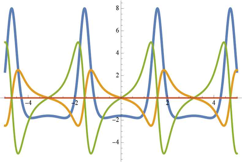
3.1.2. Localized Breather Solitons

Theorem 3.2.

If λ₀ ≠ 0 then for any fixed t the graph of the solution u_α,β,λ as a function of x will be localized in a small neighborhood of

x=cα,β,λ(t)=ln|α−1β|2λ0−vct(3.3)

and hence this disturbance is moving to the left with velocity vc=λ02−3λ12. Moreover, if λ₁ ≠ 0 then the solution will also exhibit fluctuations moving to the left at velocity vp=3λ02−λ12, giving it the “throbbing” appearance of a breather soliton.

Proof.

The squared amplitude of the solution u_α,β,λ can be written in the form

|uα,β,λ(x,t)|2=C1(|α|2eΛ+|β|2e−Λ+C2cos(Θ)+C3sin(Θ))2

If λ₀ > 0 then for sufficiently large values of |x| this amplitude converges quickly to 0. In this sense, we can already see that the solution is localized when λ has a non-zero real part. Moreover, if we “average out” the small variation from the trigonometric functions by setting them both equal to zero, then this amplitude function has a unique local maximum located at x = c_α,β,λ (t).

So, in the case λ₀ > 0 an animation of the solution u_α,β,λ (x,t) as a function of x with t playing the role of time will show a localized disturbance centered at x = c_α,β,λ (t) and traveling to the left with velocity v_c. However, if λ₁ > 0 as well, then the formula for the solution will also involve at least one of the functions cos(θ) or sin(θ). Since θ is a function of x + v_pt, these features will be moving to the left at velocity v_p. If it were the case that v_c = v_p, then the waveform would simply translate in time. However, there are no real solutions to 3λ02−λ12=λ02−3λ12 and so whenever λ₀ and λ₁ are both non-zero, an animation of the solution will exhibit the “breathing” phenomenon.

Example 3.2.

Consider the case α = j, β = 1 + k and λ=1+3i. We expect to see a localized disturbance traveling to the left with velocity v_c = −8 (which means it will move to the right with speed 8 as t increases). Moreover, since v_p = 0 all of the trigonometric function in the formula for u_α,β,λ (x,t) have arguments that are independent of t. At time t we would expect to see the center of the localized hump being located at x = 8t + ln(2)/4 (just slightly to the right of x = 8t). And this is what we see in the figures showing this solution at times t = −1 and t = 1.

3.1.3. Singularities

Either the periodic or breather soliton solutions can exhibit singularities. The following result completely identifies the values of the parameters α, β and λ that produce entirely non-singular solutions. A surprising corollary is that any of these solutions exhibiting singularities must be inherently commutative in that it is conjugate to a complex-valued solution of the standard KdV equation.

Theorem 3.3.

The quaternion-valued KdV solution u_α,β,λ (x,t) is non-singular for all x and t if any of these three conditions involving the number q = α⁻¹β is satisfied:

I.

q22+q32>0 (i.e. q is not a complex number)
II.

λ₀ = 0 and |q| ≠ 1 or
III.

λ₁ = 0 and q is not a negative real number.

Moreover, the solution u_α,β,λ (x,t) is undefined for some (x,t) ∈ ℝ² if none of the conditions is satisfied.

Proof.

Throughout Section 3.1 it has been assumed that αβ λ ≠ 0. Hence, we know that α is invertible. Define q = α⁻¹β and note that by Lemma 2.4 we know that u_1,q,λ = α⁻¹u_α,β,λ α. One of these solutions is singular if and only if the other is. Consequently, it is sufficient to determine when the solution u_1,q,λ is singular.

Since ϕ_1,q,λ is infinitely differentiable for all x and t regardless of the values of the parameters, the only way that u_1,q,λ given by (2.5) could fail to be defined and differentiable at (x₀,t₀) is if |ϕ_1,q,λ |(x₀,t₀) is zero. Using the previous notation that vp=3λ02−λ12, vc=λ02−3λ12and now defining θ = 2λ₁(x + v_pt) we find

|ϕ1,q,λ(x,t)|2=(q0+e2λ0(x+vct)cos(θ))2+(q1+e2λ0(x+vct)sin(θ))2+q22+q32.(3.4)

This sum of the squares of four real numbers can only be zero if all four of them are equal to zero.

If condition I is met then the last two terms in (3.4) are non-zero and the solution must be non-singular.

Now suppose condition II is met. Since λ₀ = 0 the exponential terms are equal to 1 and (3.4) reduces to (q0+cos(θ))2+(q1+sin(θ))2+q22+q32. However, this is only zero if (−q₀,−q₁) are the coordinates of the point at angle θ radians on the unit circle. Since |q| ≠ 1 that cannot be true.

And, if condition III is met then θ = 0 and (3.4) becomes

|ϕ1,q,λ(x,t)|2=(q0+e2λ0(x+vct))2+q12+q22+q32.

If q is not a real number then q12+q22+q32>0 and the expression is non-zero And if q is a nonnegative real number then the first term is positive for all values of x and t.

This shows that the solution is entirely non-singular if any one of the three conditions is met. Now, assume that none of the conditions is satisfied. So, we know that q22+q32=0, that either (i) λ₀ ≠ 0 or that (ii) |q| = 1, and that either (iii) λ₁ = 0 or that (iv) q is negative.

Assuming (i) and (iii) ensures that the function in the exponent and the trigonometric argument θ are linearly independent linear functions of the variables x and t and hence can be simultaneously solved to take any desired value. The point (−q₀,−q₁) is on a circle of radius |q| around the origin and hence can be written as (|q|cos(θ₀),|q|sin(θ₀)) for some value of θ. Then one can simultaneously find values of x and t such that e^{2λ₀(x+v_ct)} = |q| and θ = θ₀ thereby making the entire expression equal to zero.

If (i) and (iv) are assumed to be true then q is a negative real number and we want to show that

(q+e2λ0(x+vct)cos(θ))2+(e2λ0(x+vct)sin(θ))2

is zero for some choice for x and t. If θ = 0 then the second term is already zero and if not then a value of t can be found to make it zero. Either way the expression then reduces to (q + e^2λ₀(x+C))² for some constant C and the expression is equal to zero at x =(ln(−q) −C)/(2λ₀) (which is a real number as a consequence of (i) and (iv)).

Now suppose that (ii) and (iii) are true. We can further assume that λ₀ = 0 because otherwise (i) is true and we already handled that case. But then the expression reduces to (q₀ + cos(θ))² +(q₁ + sin(θ))². By assumption (ii), we know that the point (−q₀,−q₁) lies on the unit circle and hence there is a number θ₀ such that it is equal to (cos(θ₀),sin(θ₀)). Since λ₁ ≠ 0 it is possible to choose x and t so that θ = θ₀ and the expression then becomes zero.

Finally, consider the case in which (ii) and (iv) are both true. If λ₀ ≠ 0 is also true then that would mean (i) and (iv) are true, and it has already been demonstrated that the solution is singular in that case. On the other hand, if λ₀ = 0 then λ₁ ≠ 0 (because λ ≠ 0 is assumed throughout this section), but then (ii) and (iii) are true which has also already been handled.

Remark 3.1.

One might guess from Figure 2 that the breather soliton solution in Example 3.2 is singular because it appears to have a pole in the bottom figure. However, α⁻¹β = −i − j is not a complex number and hence according to Theorem 3.3 it is not. (In fact, redrawing the graph at time t = 1 over a larger vertical range confirms that there is simply a local maximum that is outside of the viewing window in Figure 2.)

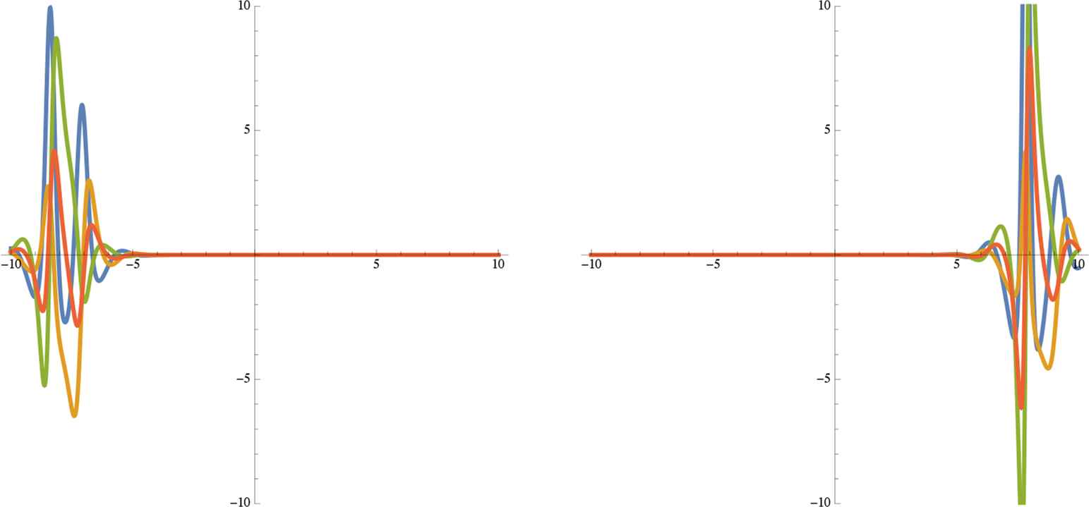
Example 3.3.

The periodic solution shown in Example 2.1 is non-singular because α = 1+k, β = 1 and λ = i so q = α⁻¹β = 1/2−1/2k which satisfies criterion II. On the other hand, choosing α = 1, β=1/5−2/5i and λ = i results in a singular solution u_α,β,λ (x,t) since none of the conditions are satisfied. This particular solution may seem uninteresting as it is complex-valued and therefore not inherently non-commutative, but it will play an important role in Example 4.2 below.

Surprisingly, it turns out that u_α,β,λ has singularities only when the solution is really commutative:

Corollary 3.1.

If the solution u_α,β,λ (x,t) is singular then u(x,t)= α⁻¹u_α,β,λ α is a complex-valued function, and u_α,β,λ is a solution of the usual KdV equation (1.1).

Proof.

If u_α,β,λ (x,t) is singular then q = α⁻¹β ∈ ℂ must be a complex number (else Condition I of Theorem 3.3 is met and the solution would be non-singular). Note that ϕ_1,q,λ = α⁻¹ϕ_α,β,λ. By Lemma 2.4

u1,q,λ(x,t)=α−1uα,β,λ(x,t)α=u(x,t)

is another solution to (1.2). However, since q and λ are both complex numbers, ϕ_1,q,λ and therefore u_1,q,λ which can be computed from it using (2.5) are complex-valued functions. Consequently u and u_x commute. Commutativity is preserved by conjugation so u_α,β,λ also commutes with its derivative. Then, both of these functions solve (1.1).

3.2. Rational Solutions

Definition 3.1.

Let ψ₀(x,t,z)= e^xz+^tz³ and for m = 0,1,2,... define Δ_m(x,t) to be

Δm(x,t)=∂mψ0∂zm|z=0.

Note that Δ_m(x,t) ∈ 𝕑[x,t] is a polynomial in x and t with integer coefficients and that it has degree m as a polynomial in x.

Theorem 3.4.

For any n ∈ ℕ and αj ∈ 𝔿, Φ = {ϕ₀,...,ϕ_n} is a KdV-Darboux kernel where

ϕ1(x,t)=∂2i∂x2i(Δ2n+1(x,t)+∑j=0nΔ2j(x,t)αj).

The corresponding quaternion-valued KdV solution u_Φ(x,t) is a rational function.

Proof.

Because

by linearity each function ϕ_i also satisfies the dispersion condition of Definition 2.1.

For i < n, (ϕ_i)_xx = ϕ_i+₁ ∈ Φ. On the other hand, ϕ_n is the (2n)^th derivative of a polynomial of degree 2n + 1, and so it is a linear function of x. Then (ϕ_n)_xx = 0 ∈ span(Φ). Thus Φ satisfies the closure property for KdV-Darboux Kernels.

Finally, to demonstrate the invertibility of the Wronskian matrix W, we consider a linear combination

∑i=0nϕiαi

of the entries in its first row with quaternionic coefficients on the right. Suppose that not all of the coefficients in this linear combination are zero and let j be the smallest value of i for which α_i = 0. Then, since ϕ_i is a polynomial in x of degree 2(n − i)+ 1 the x^2(n−j)+1 term which comes from ϕ_jα_j cannot be cancelled by any other terms in the sum. Then the linear combination is not equal to zero unless all of the coefficients are zero and the homogenous vector equation Wv = 0 has no non-trivial solutions which implies the invertibility of the matrix [27].

Since Φ is a KdV-Darboux kernel we know that u_Φ is a KdV solution and (2.4) shows that it can be found through products, and sums of derivatives of these polynomials followed by division by a real-valued polynomial and hence each component function is a rational function of x and t.

Example 3.4.

The first example of a quaternion-valued KdV solution above in Example 2.1 was an instance of this construction in the case n = 1, α₀ = k and α₁ = i.

Remark 3.2.

In fact, one may choose any finite linear combination of the polynomials Δ_m(x,t) and create a KdV-Darboux kernel out of this polynomial and all of its non-zero, even order derivatives in x. However, due to Lemmas 2.2 and 2.3, no new KdV solutions would be gained by considering even degree polynomials in Φ or including lower order odd degree terms in the formula for ϕ_i. (See [24] for details.)

4. Unions of KdV-Darboux Kernels

Since the dispersion and closure properties of Definition 2.1 are preserved under the taking of unions, it follows immediately that:

Theorem 4.1.

If Φ₁ and Φ₂ are KdV-Darboux kernels then Φ = Φ₁ ∪ Φ₂ is also a KdV-Darboux kernel as long as its Wronskian matrix is invertible.

This way of combining KdV-Darboux kernels allows for the creation of n-soliton solutions or hybrids that exhibit features of more than one of the basic solution types described in the previous section. For example, there is a rational-periodic hybrid solution coming from the union of the KdV-Darboux kernels in Examples 2.1 and 3.1.

The main focus of this section will be the case in which one additional function of the form ϕ_α,β,λ with λ₀ > 0 is added to a KdV-Darboux kernel. It is a consequence of Lemma 2.3 that the resulting solution will look like two different solutions “glued” together, one visible to the left of the localized disturbance that has been added and other other to the right of it. This general fact will be both proved and illustrated in Section 4.1. Then in Section 4.2 it will be used to derive a formula for the phase shift of an arbitrary 2-soliton solution.

4.1. Asymptotics to the Left and Right of a Localized Disturbance

Proposition 4.1.

Let Φ = {ϕ₁,...,ϕ_n} be a KdV-Darboux kernel where n ⩾ 2 and ϕ_n has the form

ϕn(x,t)=ϕα,β,λ(x,t)=αeλx+λ3t+βe−λx−λ3t

with λ = λ₀ + λ₁i, λ₀ > 0. Then for each fixed t and far enough to the left of x = c_α,β,λ (t) the graph of u_Φ(x,t) looks like^b the graph of u_ΦL (x,t) where

ΦL={QL(ϕ1),…,QL(ϕn−1)}

with Q^L(f)= f_x + βλβ ⁻¹ f. Similarly, for each fixed t and far enough to the right of x = c_α,β,λ (t) the solution u_Φ(x,t) looks like u_Φ^R (x,t) where

ΦR={QR(ϕ1),…,QR(ϕn−1)}

with Q^R(f)= f_x − αλ α⁻¹ f.

Proof.

The “center” c_α,β,λ (t) is the value of x for which there is a balance between the magnitude of the two exponential terms in ϕ_n. For x much smaller than it, αe^λx+^λ³t is negligibly small. For those values of x, the solution u_Φ(x,t) will not look noticeably different than it would if ϕ_n was equal to β e^−λx−^λ³t, which according to Lemma 2.3 is precisely u_ΦL. Similarly, when x is much larger than c_α,β,λ (t) the term β e^−λx−^λ³t is negligibly small and the solution would not look noticeably different than it would if that term was not there, which is u_ΦR according to Lemma 2.3.

Example 4.1.

Consider the “hybrid” rational/soliton solution u_Φ that comes from the choice

Φ={x+3k,ϕα,β,λ} with α=1,β=j,λ=2+i.

According to Proposition 4.1 the left side of this solution should look like

uΦL=−50x2−40x+444(5x2+4x+46)2+(5x+2)(5x2+4x+46)2+(4i+48j+36k)

and the right side should like look

uΦR=−50x2−40x+444(5x2+4x+46)2+(5x+2)(5x2+4x+46)2+(4i+48j+36k)

Each of these is a stationary (t-independent) quaternion-valued KdV solution. They are shown in the left-most and right-most images of Figure 3 respectively. The middle two images of that figure show u_Φ at times t = −5 and t = 5. Then we can see that u_Φ looks like u_ΦL to the left of the incoming soliton and looks like u_ΦR to the right of it.

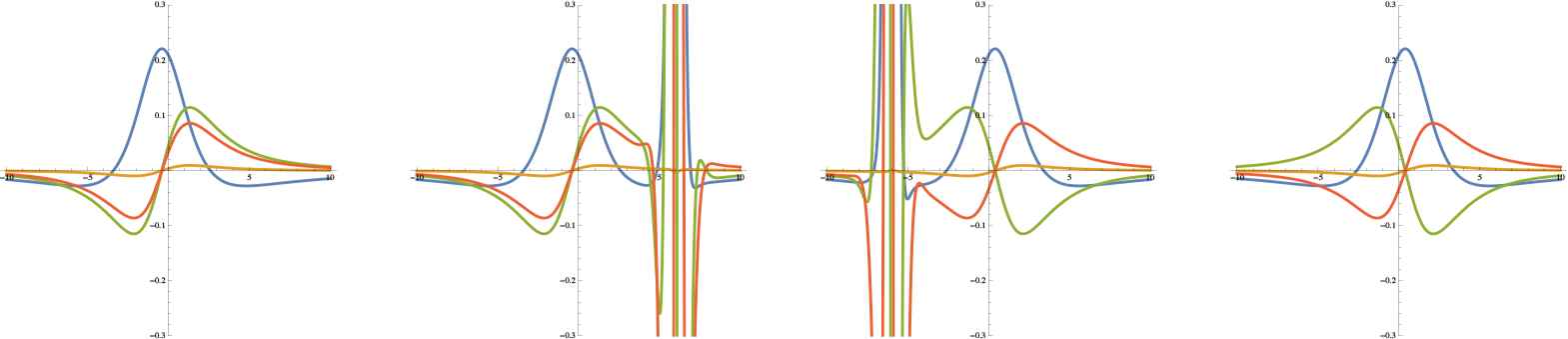
Remark 4.1.

Since Proposition 4.1 will mostly be applied in the case that each ϕ_i ∈ Φ is a function of the form (3.1), it is worth noting that the differential operator Q defined by Q(f) = f_x − γf preserves that form. In particular, it can easily be computed that for any α^,β^,λ^∈𝔿

Q(ϕα^,β^,λ^)=ϕα˜,β˜,λ˜ where α˜=α^λ^−γα^,β^=−β^λ^−γβ^.(4.1)

Example 4.2.

Let Φ₁ be the KdV-Darboux kernel

Φ1={ϕα1,β1,λ1} where α1=1,β1=15,λ1=i

then u_Φ₁ is a complex-valued, non-singular, periodic solution to (1.2). And let Φ₂ be the KdV-Darboux kernel

Φ2={ϕα2,β2,λ2} where α2=i+j,β2=j+k,λ2=1+i

so that u_Φ₂ is a breather soliton solution traveling to the right at speed 2. What will the solution coming from Φ = Φ₁ ∪ Φ₂ look like? According to Proposition 4.1 and Remark 4.1, to the left of x = c_α₂_,β_₂_,λ₂ = 2t should look like u_{α_L},_{β_L}_,λ₁ with

αL=1, βL=15−25i

while on the right it should look like u_{α_R,β_R,λ₁} where

αR=−1+i−j, βR=−15−15i−15j.

The interesting thing about this is that since |β_L| = 1 ≠ |β_R| the solution it looks like on the left is singular while the one on the right is not. Figure 4 shows that the solutions appear as predicted. Moreover, this solution is very interesting to watch as an animation because the localized disturbance traveling to the right seems to transform a non-singular periodic solution into a singular one as it passes.

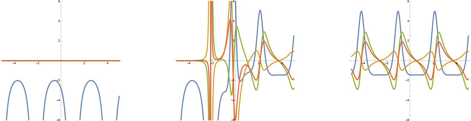
4.2. Phase Shift of the General 2-soliton

Suppose α, β, α^ and β^ are non-zero quaternions and that λ and λ^ are complex numbers such that:

λ0>0, λ^0>0, and λ^02−3λ^12<λ02−3λ12.

Then u_α,β,λ and uα^,β^,λ^ are each quaternion-valued 1-soliton solutions to (1.2). Moreover, because of the last inequality they have different velocities. In particular, the center c_α,β,λ (t) moves to the left more quickly than cα^,β^,λ^(t) (or, equivalently, moves to the right more slowly).

This section will use Proposition 4.1 to analyze the quaternion-valued KdV solution u_Φ where

Φ={ϕα,β,λ,ϕα^,β^,λ^}.

As will be seen below, there are constants α₋,β₋,α^−, β^−∈𝔿 so that an observer watching an animation of u_Φ for sufficiently negative values of t would see two localized disturbances traveling with the same velocities as c_α,β,λ and cα^,β^,λ^. In particular, there are quaternions α₋,β₋, α^−, β^−∈𝔿 so that the observer would see what appeared to be the localized disturbances from the solution u_{α₋,β₋,λ} and uα^−,β^−,λ^ together in this 2-soliton solution.

There are also numbers α₊,β₊, α^+, β^+∈𝔿 so that an animation of u_Φ for sufficiently positive values of t will look like a sum of the localized solutions u_α₊_,β₊_,λ and uα^+,β^+,λ^. So, the observer would still see two localized disturbances traveling with the same velocities. However, they might not be in the locations that the observer would have predicted. Suppose the observer identifies the localized disturbances of the same velocities at different times. Then, since at negative times the disturbance with greater velocity appears to be following the linear trajectory c_{α₋,β₋,λ} (t), the observer may expect it to be found on that same line at positive times as well. Indeed, since c_{α₋,β₋,λ} and c_{α₊,β₊,λ} (t) are moving to the left at the same velocity, their difference is a constant. If it is zero, then the observer will find that the disturbance at later times is right where it would have been expected to be. However, if this difference is non-zero, then it will be shifted from its expected position. Hence, the number c_{α₊,β₊,λ} − c_{α₋,β₋,λ} is called the phase shift of that localized disturbance and it is generally interpreted as being a lasting consequence of its collision with the other localized disturbance (though there are other interpretations as well) [2, 26].

The following result provides formulas for the parameters for the corresponding 1-soliton solutions and the phase shifts of each of the localized disturbances. As the examples after it demonstrate, unlike the real case, the phase shift of the solitary wave with greater velocity in the quaternion-valued KdV 2-soliton can be positive, negative, or zero. Additionally, the solitary waves traveling at the same velocities at positive and negative may differ in shape as well as being horizontally shifted relative to each other.

Proposition 4.2.

Choose constant α, β, λ, α^,β^, and λ^ as described above and let Φ be the KdV-Darboux kernel

Φ={ϕα,β,λ,ϕα^,β^,λ^}.

For sufficiently negative values of t, the solution u_Φ will look like the 1-soliton u_{α₋,β₋,λ} near its center x = c_{α₋,β₋,λ} (t) and will also look like the 1-soliton uα^−,β^−,λ^ near its center x=cα^−,β^−,λ^(t) where
α−=αλ−α^λ^α^−1α,β−=−βλ−α^λ^α^−1β,α^−=α^λ^+βλβ−1α^,andβ^−=−β^λ^+βλβ−1β^.
For sufficiently positive values of t, the solution u_Φ will look like the 1-soliton u_α₊_,β₊_{,_λ} near its center x = c_α₊_,β₊_,λ (t) and will also look like the 1-soliton uα^+,β^+,λ^ near its center x=cα^+,β^+,λ^(t) where
α+=αλ+β^λ^β^−1α,β+=−βλ+β^λ^β^−1β,α^+=α^λ^−αλα−1α^,andβ^+=−β^λ^−αλα−1β^.
The phase shifts experienced by the interacting solitary waves are
cα+,β+,λ(t)−cα−,β−,λ(t)=ln(γ)2λ0 and cα^+,β^+,λ^(t)−cα^−,β^−,λ^(t)=ln(γ)2λ^0

where

γ=|αλα−1−α^λ^α^−1||βλβ−1−β^λ^β^−1||αλα−1−β^λ^β^−1||βλβ−1−α^λ^α^−1|.

Proof.

First, we will apply Proposition 4.1 to Φ using ϕα^,β^,λ^ in the role of ϕ_n. The proposition says that for all t, far enough to the right of cα^,β^,λ^(t), the graph of the solution u_Φ will look like u_{α₋,β₋,λ} using the values from above. Because the center c_{α₋,β₋,λ} (t) is moving to the left more quickly, for any sufficiently negative value of t, it will be far enough to the right of cα^,β^,λ^ so that it is in the region where u_Φ looks like u_{α₋,β₋,λ}. Therefore for very negative values of t, u_Φ has a localized disturbance that looks like the one in the one soliton u_{α₋,β₋,λ}.

On the other hand, when t is very positive then c_α₊_,β₊_,λ (t) will be far to the right of cα^,β^,λ^(t).In particular, because it is moving to the left at a faster constant speed when t is sufficiently large it will be located in the region where according to Proposition 4.1 the solution u_Φ will look like u_α₊_,β₊_,λ. Since that is the location around which the soliton is localized in that 1-soliton, the solution u_Φ will look like that 1-soliton near that point.

The other parameters come from repeating this same process but now using ϕ_α,β,λ in the role of ϕ_n when applying Proposition 4.1.

Now, c_α₊_,β₊_,λ (t) and c_{α₋,β₋,λ} (t) are two linear trajectories with the same velocity. The difference between them is the phase shift, how much further to the right the disturbance is after the collision than it would have been if it had continued to look like u_{α₋,β₋,λ}. Using the formula for the center, properties of logarithms and properties of the length operator on quaternions, we can see that

cα+,β+,λ(t)−cα−,β−,λ(t)=ln|α+−1β+|2λ0−ln|α−−1β−|2λ0=12λ0ln(|α+−1β+||α−−1β−|)=12λ0ln(|α−||β+||α+||β−|)=12λ0ln(|αλ−α^λ^α^−1α||−βλ+β^λ^β^−1β||αλ−β^λ^β^−1α||−βλ+β^λ^β^−1β|)=12λ0ln(|αλα−1−α^λ^α^−1||βλβ−1+β^λ^β^−1||αλα−1+β^λ^β^−1||βλβ−1+α^λ^α^−1|)=ln(γ)2λ0.

A similar calculation for cα^+,β^+,λ^−cα^−,β^−,λ^ results in the same formula but with the numerator and denominator switched in the argument of the logarithm with the effect of changing the sign.

Example 4.3.

Imagine a naive observer watching an animation of the 2-soliton solution u_Φ where Φ={ϕα,β,λ,ϕα^,β^,λ^} with

α=β=α^=1,β^=20i+k,λ=2+i,λ^=3/2+3/2i

Watching for some negative values of t, the observer would see a stationary breather soliton sitting just a bit to the right of x = 0 and then another breather soliton approaching from the right at speed 1. In fact, as predicted by Proposition 4.2 the moving soliton looks like u_{α₋,β₋,λ} as shown at the top-left of Figure 5. In particular, for these negative times, the moving localized disturbance in u_Φ is located at

x=cα−,β−,λ(t)=log(31+163)8−t.

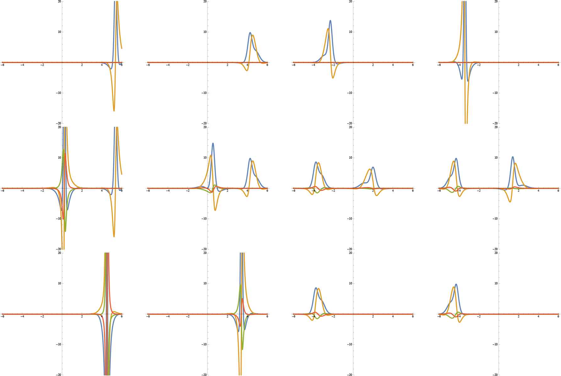
So, the naive observer might assume that this will continue to be true in the future. However, as the images on the right in Figure 5 show, it does not. Although there is still a disturbance moving left at speed 1 at times t = 3 and t = 4, it no longer looks like u_{α₋,β₋,λ}. Instead, it looks like u_α₊_,β₊,λ, a 1-soliton whose center is:

x=cα+,β+,λ(t)=18log(711433−36571234434199)−t.

Since they are both traveling to the left at the same speed, their difference is a constant

cα+,β+,λ−cα−,β−,λ=18log(39608599−227200003855800407)≈−1.01413,

which means that the observer would find the localized disturbance after the collision is about 1.014 units farther to the left than expected. (Similarly, the phase shift for the stationary soliton would be positive, which is why it has moved to the right after the interaction.)

Remark 4.2.

The phase shift experienced by each of the two solitary waves experience have opposite signs. Like the classical commutative KdV solitons, if one is shifted forwards then the other shifts backwards. However, unlike the original KdV solitons studied by Zabusky and Kruskal [26], the phase shift is not completely determined by the velocities, as the next example illustrates.

Example 4.4.

A one parameter family of interesting examples is the case in which

α=1,β=1,λ=1+3i,α^=j,β^=i+ck,andλ^=1+4i.

For any value of c ∈ ℝ this represents a 2-soliton solution with one traveling to the right at speed 26 and another at speed 47. However, the phase shift that they experience depends on c:ln(γ) is positive for |c|>1/11, zero if |c|=1/11 and negative if |c|<1/11. This dramatically demonstrates the fact that in the non-commutative case the phase shift depends on the coefficients α, β,α^ and β^. That does not happen in the commutative case, as one can observe by noting that all dependence on these coefficients cancel from the formula for γ in Proposition 4.2 if the parameters commute.

5. Concluding Remarks

Although it is surely no more than a coincidence that the quaternions and the existence of solitary waves were both famously discovered beside British canals in the 19th century, this paper has found interesting results by studying quaternion-valued solutions to the KdV-equation that can be produced using the Chen determinant. This is both a generalization of and a special case of other published research, as will be explained further below.

When the functions in the KdV-Darboux kernel Φ are all either complex-valued or real-valued, then the solution u_Φ satisfies (1.1) and many of the new results in this paper reduce to well-known results. For instance, singularities of soliton and periodic complex-valued solutions to KdV have been studied in Reference [21] much as we considered the singularities of the quaternion-valued solutions in Theorem 3.3. However, the generalization to the non-commutative case handled here is non-trivial. Without Corollary 3.1 it was not at all obvious that the singularities that can be found in complex-valued KdV solutions would necessarily fail to exist in their non-commutative quaternionic counterparts. Moreover, as noted in Example 4.4, the phase shift in the quaternion-valued 2-soliton depends on the coefficients as well as on the exponents, something that is not true in the commutative case.

On the other hand, there are also many published papers which address non-commutative solutions to integrable PDEs in more general settings. The KdV equation is merely one equation in the KdV hierarchy, which is a reduction of the KP hierarchy. Quaternions can be viewed as being a special four-dimensional subspace of larger matrix groups, which are then special cases of abstract non-commutative rings. With all of that in mind, the methods utilized herein can be seen as simply being a special case of the more general approaches found in papers such as References [3 ,6,9,23]. However, limiting ourselves to this manageable situation allows us to study details that would be difficult to notice and demonstrate in those more general settings. For instance, we were able to show that it was sufficient to consider exponential functions of the form e^λx+^λ³t where λ = λ₀ + λ₁i is a complex number with non-negative components λ_i (cf. Lemma 3.1). Doing so was essential in being able to state Theorem 3.3 (the result about singularities) in an easily understandable way. And, since 𝔿 is a four-dimensional vector space, we were able to graph the corresponding solutions as a super-position of graphs of four real-valued functions. Moreover, it is interesting to know that quaternion-valued solutions to KdV can be written in terms of the Chen determinant, a result that presumably would not generalize to solutions with values in arbitrary non-commutative rings.

There is one relatively recent paper by Huang [12] which, like this one, specifically addresses quaternion-valued soliton solutions to KdV. However, Huang’s paper only considers a small subset of the solution types that were addressed above. In particular, it only looks at solutions that would come from KdV-Darboux kernels made up of functions of the form ϕ_α,β,λ where α,β ∈ 𝔿 and λ ∈ ℝ. Thus, it does not include breather, rational, or periodic solutions. Finally, although Reference [12] does discuss “interactions” of the solutions, that term has a very different meaning in that paper. Here, Proposition 4.1 is viewed as a means to understand the interaction of different solutions, with special emphasis on the 2-soliton solutions as representing the interaction between two separate 1-solitons (cf. Proposition 4.2). But in Reference [12], “interaction” refers to an algebraic structure that Huang studies whereby two n-solitons can be combined to produce another n-soliton (for the same fixed value of n).

There are many interesting examples which can be made using the methods described above that we did not have the time or space to present here. For instance, there are 2-soliton solutions that look like a combination of non-singular 1-solitons at negative times and then like a pair of singular 1-solitons for positive times (as if the collision produced the singularities).

There are also open problems that we have not been able to fully address. Theorem 3.3 completely determines when a solution of the form u_α,β,λ is singular. However, it is not entirely clear when combinations of such solutions are singular. Although Propositions 4.1 and 4.2 may tell us when they look singular, as Remark 3.1 shows, that is not quite the same as actually being singular. We do not yet have any prediction for what u_Φ will look like if Φ = {ϕ_α₁_,β₁_,λ₁,...,ϕ_{α_n,β_n,λ_n}} with n > 1 and λ_i = λ_i1i purely imaginary. Most intriguingly, since the solutions above were written in terms of the Chen determinant of a Wronskian matrix, it would be interesting to know whether there is a quaternionic analogue of the τ-function and Hirota’s bilinear approach to soliton equations.

Acknowledgments

This paper grew out of a student research project at the College of Charleston conducted in Summer 2018. The first author’s research was supported by a grant from the School of Sciences and Mathematics, the third author’s research was supported by the University of Charleston, South Carolina (the Graduate School at the College of Charleston), and the fourth author’s research was supported by a Summer Undergraduate Research with Faculty (SURF) grant from the Office of Undergraduate Research and Creative Activities. Assistance from all of these offices and from the Department of Mathematics at the College of Charleston is greatly appreciated.

Footnotes

a

The quasi-determinant [6] is useful in non-commutative settings. However, it is not a generalization of the determinant in that a quasi-determinant of a matrix which happens to have commuting entries is not equal to the determinant of that matrix.

b

We are being intentionally vague about what it means for one solution to “look like another” to the right or left of some value of x here because the notation and proofs both become unwieldy otherwise. A rigorous mathematical definition might include an arbitrarily small maximum amplitude for the difference of the two functions when x is is more than a certain distance to the right or left of c_α,β,λ (t). It is hoped that Examples 4.1 and 4.2 illustrate both the meaning and significance of Proposition 4.1.

References

[1]S.L. Adler, Quaternionic Quantum Mechanics and Quantum Fields, Oxford University Press, New York, 1995.

[2]N. Benes, A. Kasman, and K. Young, On Decompositions of the KdV 2-Soliton, Journal of Nonlinear Science, Vol. 16, No. 2, 2006, pp. 179-200.

[3]S. Carillo, M. Lo Schiavo, E. Porten, and C. Schiebold, A novel noncommutative KdV-type equation, its recursion operator, and solitons, J. Math. Phys, Vol. 59, 2018, pp. 043501.

[4]L. Chen, Definition of Determinant and Cramer Solutions over the Quaternion Field, Acta Mathematica Sinica, New Series, Vol. 7, No. 2, 1991, pp. 171-180.

[5]J.H. Conway and D.A. Smith, On Quaternions and Octonions, AK Peters/CRC Press, 2003.

[6]P. Etingof, I. Gelfand, and V. Retakh, Factorization of differential operators, quasideterminants, and nonabelian Toda field equations, Mathematical Research Letters, Vol. 4, No. 3, 1997, pp. 413-425.

[7]J.D. Gibbon, A quaternionic structure in the three-dimensional Euler and ideal magnetohydrodynamics equation, Physica D, Vol. 166, 2002, pp. 17-28.

[8]P.R. Girard, Quaternions, Clifford algebras and relativistic physics, Birkhäuser Verlag, Basel, 2007. Translated from the 2004 French original

[9]M. Hamanaka and H. Okabe, Soliton Scattering in Noncommutative Spaces, Theor. Math. Phys, Vol. 197, 2018, pp. 1451.

[10]W.R. Hamilton, On Quaternions; or on a new System of Imaginaries in Algebra, Philosophical Magazine, Vol. xxv, 1844, pp. 10-13.

[11]D.D. Holm, Geometric Mechanics: Part 2, Rotating, Translating and Rolling (Pt. II), Imperial College Press, 2008.

[12]S. Huang, An operator method for finding exact solutions to vector Korteweg-de Vries equations, Journal of Mathematical Physics, Vol. 44, No. 3, 2003, pp. 1357-1388.

[13]A. Kasman, Glimpses of Soliton Theory, American Mathematical Society, Vol. 54, 2010.

[14]A. Kasman, On factoring an operator using elements of its kernel, Communications in Algebra, Vol. 45, No. 4, 2017, pp. 1443-1451.

[15]K. Kenatani, Understanding Geometric Algebra: Hamilton, Grassmann, and Clifford for Computer Vision and Graphics, AK Peters, 2015.

[16]D.J. Korteweg and G. de Vries, On the change of form of long waves advancing in a rectangular canal, and on a new type of long stationary waves, The London, Edinburgh, and Dublin Philosophical Magazine and Journal of Science, Vol. 39, No. 240, 1895, pp. 422-443.

[17]K.I. Kou, W.-K. Liu, and Y.-H. Xia, Solve the linear quaternion-valued differential equations having multiple eigenvalues, Journal of Mathematical Physics, Vol. 60, 2019, pp. 023510.

[18]I.I. Kyrchei, Cramer’s rule for quaternionic systems of linear equations, Journal of Mathematical Sciences, Vol. 155, No. 6, 2008, pp. 839-858.

[19]S. Leo, G. Ducati, and C. Nishi, Quaternionic potentials in non-relativistic quantum mechanics, J. Phys. A: Math. Gen, Vol. 35, No. 26, 2001, pp. 5411.

[20]S. Leo and G. Ducati, Solving simple quaternionic differential equations, J. Math. Phys, Vol. 44, No. 5, 2003, pp. 2224.

[21]Y.C. Li, Simple explicit formulae for finite time blow up solutions to the complex KdV equation, Chaos Solitons and Fractals, Vol. 39, 2009, pp. 369-372.

[22]R. Palais, Symmetries of Solitons Bulletin (New Series) of the American Mathematical Society, Vol. 34, No. 4, October 1997, pp. 339-403.

[23]L.D. Paniak, Exact Noncommutative KP and KdV Multi-solitons.

[24]A. Serna, Quaternion-valued Rational Solutions to the KdV Equation, College of Charleston, 2019. Master’s Thesis

[25]P. Wilczynski, Quaternionic-valued ordinary differential equations. II. Coinciding sectors, J. Differ. Equations, Vol. 252, 2012, pp. 4503-4528.

[26]N. Zabusky and M. Kruskal, Interaction of “Solitons” in a Collisionless Plasma and the Recurrence of Initial States, Phys. Rev. Lett, Vol. 15, 1965, pp. 240.

[27]F. Zhang, Quaternions and matrices of quaternions, Linear Algebra and Its Applications, Vol. 251, 1997, pp. 21-57.

<Previous Article In Issue

Download article (PDF)

Next Article In Issue>

Journal: Journal of Nonlinear Mathematical Physics
Volume-Issue: 27 - 3
Pages: 429 - 452
Publication Date: 2020/05/04
ISSN (Online): 1776-0852
ISSN (Print): 1402-9251
DOI: 10.1080/14029251.2020.1757234 How to use a DOI?
Open Access: This is an open access article distributed under the CC BY-NC 4.0 license (http://creativecommons.org/licenses/by-nc/4.0/).

Cite this article

ris enw bib

TY  - JOUR
AU  - John Cobb
AU  - Alex Kasman
AU  - Albert Serna
AU  - Monique Sparkman
PY  - 2020
DA  - 2020/05/04
TI  - Quaternion-Valued Breather Soliton, Rational, and Periodic KdV Solutions
JO  - Journal of Nonlinear Mathematical Physics
SP  - 429
EP  - 452
VL  - 27
IS  - 3
SN  - 1776-0852
UR  - https://doi.org/10.1080/14029251.2020.1757234
DO  - 10.1080/14029251.2020.1757234
ID  - Cobb2020
ER  -

download .riscopy to clipboard