The Group-Theoretical Analysis of Nonlinear Optimal Control Problems with Hamiltonian Formalism

Gülden Gün Polat; Teoman Özer

doi:10.1080/14029251.2020.1683985

<Previous Article In Issue

Download article (PDF)

Next Article In Issue>

Volume 27, Issue 1, October 2019, Pages 106 - 129

The Group-Theoretical Analysis of Nonlinear Optimal Control Problems with Hamiltonian Formalism

Authors

Gülden Gün Polat

Department of Mathematics and Computer Science, İstanbul Kültür University, Bakırköy, İstanbul, 34156 Turkey,g.polat@iku.edu.tr

Teoman Özer^*

Department of Civil Engineering, İstanbul Technical University, 34469 Maslak, İstanbul, Turkey,tozer@itu.edu.tr

^*Corresponding author

Corresponding Author

Teoman Özer

Received 27 December 2018, Accepted 12 July 2019, Available Online 25 October 2019.

DOI: 10.1080/14029251.2020.1683985 How to use a DOI?
Keywords: Nonlinear optimal control problems; theory of Lie groups; dynamic optimization; Hamiltonian formalism; Pontryagin’s maximum principle; economic growth models
Abstract: In this study, we pay attention to novel explicit closed-form solutions of optimal control problems in economic growth models described by Hamiltonian formalism by utilizing mathematical approaches based on the theory of Lie groups. For this analysis, the Hamiltonian functions, which are used to define an optimal control problem, are considered in two different types, namely, the current and present value Hamiltonians. Furthermore, the first-order conditions (FOCs) that deal with Pontrygain maximum principle satisfying both Hamiltonian functions are considered. FOCs for optimal control in the problem are studied here to deal with the first-order coupled systems. This study mainly focuses on the analysis of these systems concerning for to the theory of symmetry groups and related analytical approaches. First, Lie point symmetries of the first-order coupled systems are derived, and then by using the relationships between symmetries and Jacobi last multiplier method, the first integrals and corresponding invariant solutions for two different economic models are investigated. Additionally, the solutions of initial-value problems based on the transversality conditions in the optimal control theory of economic growth models are analyzed.
Copyright: © 2020 The Authors. Published by Atlantis and Taylor & Francis
Open Access: This is an open access article distributed under the CC BY-NC 4.0 license (http://creativecommons.org/licenses/by-nc/4.0/).

1. Introduction

By analyzing the optimal control problems, the calculus of variations is one of the approaches constructed on the use of Lagrangian and Hamiltonian functions and the Euler-Lagrange equations [4, 9, 12, 22]. An optimal control problem is modeled with a state variable describing the state of the system at any point in time, a control variable dealing with the choice of variables and constraint function.Besides, the necessary conditions for Pontryagin’s maximum principle provide the determination of the costate variable [6, 45]. These conditions are defined via the first-order partial derivatives of the Hamiltonian function with respect to control, state, and costate variables, which are called the first-order conditions (FOCs). From the mathematical point of view, these conditions (FOCs) generate the systems of first-order ordinary differential equations (ODEs). Moreover, it can be varied with respect to the formulization of the optimal control problem. It is clear that the consideration of the current value Hamiltonian is more desirable since the maximum principle demands the differentiation of present value Hamiltonian in which the discount factor further adds complexity to the derivatives [1].

In addition to the current value Hamiltonian functions, the present value Hamiltonian functions can be considered for the analytical solutions of the optimal control problems in the study and then one can consider the first-order system of ODEs obtained via the first-order conditions in order to analyze by some novel mathematical methods, which are Lie symmetry groups, Jacobi last multiplier (JLM), and λ-symmetries and deal with the analytical solutions by considering the first integrals (or conservation laws) of the systems. The theory of Lie groups developed in the 19th century by Norwegian mathematician Sophus Lie [24] and was constructed to investigate the similarity solutions of systems of differential equations. After the studies of Lie, in the 20th century many researchers with the advancing computer technology interested in Lie theory and did important contributions to this field. In particular, [8,39] contain many references to further contributions. It is known from the Lie theory it is not possible to determine to Lie symmetries of these systems by package programs such as MathLie or GEM [5, 10] since there is no a regular procedure to determine Lie point symmetries of first-order ODEs, unlike higher-order ODEs. This is one of the difficulties to deal with symmetries of the first-order systems of ODEs. In addition, the investigation of Lie symmetries of optimal control problems can be troublesome because of the complexity of finding the solution of a corresponding overdetermined system of PDEs, called determining equations, in particular for the system of the first-order ODE.

It is known that the method of Jacobi last multiplier (JLM) and λ-symmetry have a direct relationship with Lie point symmetries. The JLM approach built up by Jacobi [19,20] for the application of the multipliers to classical mechanics problems. Moreover, he demonstrated that the JLM method could be used to determine the first integrals of second-order ODEs. The connection between Lie point symmetries and the multipliers are revealed by Sophus Lie [24]. After long years, Nucci and her workmates presented the relation of the Jacobi method with Lagrangian and multipliers [34–38]. Then the researchers have done many notable studies based on the applications of this method [13, 18, 26]. λ-symmetry approach can be considered as the other Lie point symmetry related method developed by Muriel and Romero using the definition of new prolongation formula on a λ-function [27–29, 44]. This approach includes some notable connections between the first integrals and the integrating factors of ODEs. Even though λ-symmetry was constructed for the reductions of the second-order ODEs that do not have Lie point symmetries, however, it can be said that λ-symmetry method is a quite applicable approach to obtain the reduced forms of linear or nonlinear second-order ODEs [16, 17]. The extension of λ-symmetries to PDEs, which are called μ-symmetries, are investigated in the literature [14,15,40]. Besides the theory is applied to nonlocal equations [2, 41].

In this study, we deal with some nonlinear optimal control problems arising in the theory of economics defining by an economic model. Economic modeling is at the heart of economic theory. In economics, a model is known as a theoretical construction representing economic processes by a set of variables and a set of logical and/or quantitative relationships between them [3, 42]. In addition, the model helps to isolate and sort out complicated chains of cause and effect and influence between the numerous interacting elements in an economy. The economic model is a simplified mathematical framework designed to illustrate complex processes [9]. Therefore, the most formal and abstract of the economic models are purely mathematical models. The analysis of these models is usually based on the concept of optimization under some constraints, and dynamic optimization is one of the most common applications. Dynamic optimization can be evaluated in discrete time and continuous time [1, 6]. The economic growth models in this study are formulated in the continuous time since continuous time optimization introduces a number of new mathematical issues. In continuous time, dynamic optimization has three major approaches such as dynamic programming, variation of calculus, and optimal control theory [25, 46]. Because of the complexity of most applications, the optimal control problems are most often solved by numerically in the literature. Numerical methods for solving optimal control problems back date to 1950s [6]. Over the last decades, the optimal control problems have become more difficult related to the complexity of models, so available methods have been improved. The solutions of optimal control problems have been very important for many disciplines that are financial economics, dynamic macroeconomics theory, etc. The applications of optimal control theory have been extended to growth theory by Arrow [3], Ramsey [42], Solow [45], Lucas, Uzawa and Romer [25, 43, 46] and others [1, 4, 9, 11, 12, 21, 22]. For a great majority of economic models, the integrand function contains a discount factor and in such cases, the current value Hamiltonian is more useable, which is independent of discount factor and it is more desirable in economic analysis [1, 30]. In the literature, there are some studies on optimal control problems by using the partial Hamiltonian method dealing with only the current value Hamiltonian [30–33].

In this paper, we focus on two different optimal control problems. The explicit closed-form analytical solutions based on symmetry group properties and mathematical relations related to Jacobi last multiplier and λ-symmetry methods are analyzed by considering related conditions of the models. This paper is devoted to present the applications of mathematical methods to optimal control problems to investigate not only the analytical solutions and but also the solutions of initial-value problems by organizing as follows. Section 2 consists of important properties of the mathematical methods. Section 3 includes an optimal growth model with environmental asset. Section 4 consists of the analysis of planner’s problem, which is another growth model in economics. Some considerable conclusions and discussions on the study are introduced in Section 5.

2. Preliminaries

2.1. Optimal control problems and Hamiltonian functions

Let us consider a decision problem to maximize the total profits of a firm for an interval of time t.In this problem, there are three important variable functions of time. First, q(t) is the stock of capital of a firm, c(t) is a decision function, and u = u(t,q,c) is the net profit of a firm per unit time. In order to obtain the total net profit for the terminal date T, it should be integrated for all interval of time, where the initial date is taken as t = 0, that is

W(t,q,c)=∫0Tu(t,q,c)dt,(2.1)

where W (t,q,c) is the total net profit. The main problem is to determine the decision function c(t) to make the maximum the total profit by considering the effect of the decision function on the stock of capital and the total net profit [12]. Thus, the well-known maximum principle is based on constructing a Hamiltonian function in the form

H(t,q,c)=u(t,q,c)+p(t)f(t,q,c)(2.2)

where p(t) is the marginal value of the capital at time t and f (t,q,c) is a constraint function, which is the rate of change of capital stock at any instant of time t. One of the methods is to select the decision function c(t) for a interval of time to make the Hamiltonian function as great as possible. The main idea is to find the control variable c(t) to maximize the integral (2.1) subject to the constraint

q˙(t)=dqdt=f(t,q(t),c(t)),(2.3)

with an initial condition q(0)= q₀ = constant. The functions u(t,q,c) and f (t,q,c) are assumed to be twice continuously differentiable with respect to q, differentiable with respect to c, and continuous with respect to t. One can say that if c˜(t)(t) is the solution of the problem and there is a corresponding p(t) function satisfying the relation

p˙(t)=−∂H∂q,(2.4)

so that the function c˜(t) maximizes the Hamiltonian function (2.2). In the literature, there are some methods for solving optimal control problems in the economic growth models discussed by Arrow and Kurz, Barro and Sala-i-Martin and Cass [3, 4, 9]. Most of these methods are based on a usual procedure related to the Pontryagin’s maximum principle. The goal of this principle is to satisfy some necessary conditions for optimality together with the transversality condition, required that the terminal value of costate variable has the condition p(t) ≥ 0.

In general, the optimal control problems are considered of the form

Maximize ℱ=∫0TF(t,q,c)e−ρtdt(2.5)

subject to q˙i=fi(t,q,c), i=1,…,n,(2.6)

where c =(c₁,...,c_m) is the control vector, m ≤ n or m > n with the proper boundary conditions, t is the independent variable representing the time and the pair (q, p)=(q¹,...,qⁿ, p₁,..., p_n) are the space coordinates, where q¹,...,qⁿ are called the state variables and p₁,..., p_n are called the costate variables [30]. Here the integrand in the integral (2.5) contains the discount factor e⁻^ρt. In addition, in order to construct an optimum control problem, the related Hamiltonian functions H can be regarded as two types, namely present value Hamiltonian and current value Hamiltonian functions. In general, the current value Hamiltonians are used more often in the literature to analyze the optimal control problems because of the mathematical difficulty related to the calculations with the present value Hamiltonians.

Definition 2.1.

The present value Hamiltonian is defined as

H¯=F(t,q¯,c¯)e−ρt+p¯ifi(t,q¯,c¯),(2.7)

and the current value Hamiltonian is defined by

H=F(t,q,c)+pifi(t,q,c).(2.8)

Remark 2.1.

The necessary conditions for optimal control based on the Pontryagin maximum principle for present value Hamiltonian H¯ are given by

∂H¯∂c¯i=0, ∂2H¯∂c¯i2<0,(2.9)

q˙¯i=∂H¯∂p¯i,(2.10)

p˙¯i=−∂H¯∂q¯i, i=1,…,n,(2.11)

and the necessary conditions in terms of current value Hamiltonian H are

∂H∂ci=0,(2.12)

q˙i=∂H∂pi,(2.13)

p˙i=−∂H∂qi+Γi, i=1,…,n,(2.14)

in which Γ_i is generally taken as a nonzero function of t, p_i,qⁱ and it is generally formulated as a linear function of costate variable p_i, and the time t parameter.

The conditions (2.9)–(2.11) and (2.12)–(2.14) derive optimality with all variables starting out from any given initial position. By this way, both optimal control problems and associated optimal initial values become much more simple for determining the optimality. In this study, the analysis of the optimal control problems in economic growth models is considered by taking into account both current value Hamiltonian and present value Hamiltonian functions.

2.2. The method of Jacobi last multiplier

It is known that one of the most efficient methods for the investigation of the solutions of differential equations is based on the study of Lie group of transformations. In addition, in the literature, there are some methods related to Lie symmetries such as λ-symmetry and Jacobi last multiplier, which are highly effective to obtain the reduced form of given equation in order to study the first integrals. One of them is Jacobi last multiplier method and its important relations with first integrals and multiplier for ODEs and multidimensional systems whose Lie symmetries are known [34–37].

The method of JLM enables to derive all the solutions of the partial differential equation,

Af=∑i=1nai(x1,…,xn)∂f∂xi=0,(2.15)

or its equivalent associated Lagrange’s system,

dx1a1=dx2a2=…=dxnan.(2.16)

Then the multiplier of this system M is indicated by the formula

∂(f,ω1,ω2,…,ωn−1)∂(x1,…,xn)=MAf,(2.17)

where

∂(f,ω1,ω2,…,ωn−1)∂(x1,…,xn)=det[∂f∂x1…∂f∂xn∂ω1∂x1∂ω1∂xn⋮⋮∂ωn−1∂x1…∂ωn−1∂xn]=0,

and ω₁,...,ω_n₋₁ are n − 1 solutions of (2.15) or, equivalently, first integrals of (2.16). Furthermore M is a solution of the linear PDE, which is proved by Jacobi

∑i=1n∂Mai∂xi=0.(2.18)

In addition, it can be expressed equivalently

∑i=1nai∂(logM)∂xi+∑i=1n∂ai∂xi=0,(2.19)

every solution M of this equation is a Jacobi Last Multiplier. It is clear that every different integral gives another multiplier such as M˜. Therefore, any ratio of two different multipliers M/M˜ represents a first integral of (2.16) or is a solution ω of (2.15).

Actually, the existence of a solution/first integral is a result of the existence of a symmetry, Lie in [23], presented an alternative formulation in terms of symmetries. The formulation in terms of solutions/first integrals and symmetries is pointed out by Bianchi [7]. If n − 1 symmetries of system (2.16) are known

Γi=∑j=1nξij(x1,…,xn)∂xj, i=1,…,n−1,(2.20)

then Jacobi last multiplier is represented by M = Δ⁻¹, verified that Δ ≠ 0, where

Δ=det[a1…anξ1,1ξ1,n⋮⋮ξn−1,1…ξn−1,n].(2.21)

3. Optimal Growth Model with Environmental Asset

In this part, as a first economic model of the study, the problem called an optimal growth model with an environmental asset is analyzed [21]. In this problem, the asset is evaluated as natural capital or environmental quality and it is valued both as a source of consumption of environmental services and as a stock of amenities. This model is formulated as an optimal control problem in which the social planner seeks to maximize the integral

Max ∫0∞csϕ(1−σ)1−σe−ρtdt, ϕ≥0, σ>0, σ≠1, ρ>0,(3.1)

subject to the constraint

s˙=ms−c(3.2)

in which s(t) is the stock environmental asset, c(t) is the consumption, σ is the inverse of intertemporal elasticity of substitution, φ is the relative presence for environment, m > 0 is the regeneration rate for environmental asset, and ρ is the discount factor. This model is analyzed by using the partial Hamiltonian method in the studies [31, 32] by considering only for the current value Hamiltonian function. In this section, the problem given by (3.1) and (3.2) is studied by taking account of both current and present value Hamiltonians by using the approaches of JLM, Lie point symmetries, and λ-symmetries.

Definition 3.1 (Tranversality condition).

This condition is an optimally condition often used to characterize the optimal paths (plans, programs, trajectories, etc.) of economic models. The transversality condition is essential in infinite-dimensional problems since it makes sure that there are no beneficial simultaneous changes in an infinite number of choice variables [1].

3.1. First integrals and analytical solutions for current value Hamiltonian

To obtain a solution of the problem (3.1) and (3.2), first we consider the current value Hamiltonian for the model (3.1) written via (2.8) in the form

H(t,c,s,p)=csϕ(1−σ)1−σ+p(ms−c),(3.3)

in which p(t) is the costate variable. Initially, the necessary FOCs for the optimal control problem by applying the equations (2.12)–(2.14)

p=c−σsϕ(1−σ),(3.4)

s˙=ms−c(3.5)

p˙=(σ−m−ϕcs)p,(3.6)

are determined and then the corresponding the growth rate of consumption via equations (3.4)–(3.6) is defined such that

c˙cϕ(1σ)m+ϕcs+m−pσ.(3.7)

To evaluate the solution of the optimal control problem, the appropriate initial conditions should be considered for state, control, and costate variables in the formulation of the problem. For this model, the related initial conditions are

c(0)=c0, s(0)=s0,(3.8)

and the transversality condition is given by

limt→∞e−ρtp(t)s(t)=0.(3.9)

By considering the system of coupled ODEs with the elimination of control variable c(t) from the equations (3.4)–(3.6), the related first-order system of ODEs

s˙=ms−p−1/σs(1−σ)ϕσ,(3.10)

p˙=p(−m+p−ϕp−1/σs(1−σ)ϕσ−1),(3.11)

are obtained.

Proposition 3.1.

The system of first-order coupled differential equations (3.10) – (3.11) possesses four-dimensional Lie algebra L₄.

Proof.

It can be shown that the direct integration of the determining equations in terms of t, p, and s variables gives the following four-dimensional Lie algebra L₄

X1=∂∂t, X2=−p(σ−ϕ+σϕ)∂∂p+s∂∂s,X3=∂∂t+p(1−m+p)∂∂p−s(1−m−ρ)ρ+m(σ−1)∂∂s,X4=σ(et(ρ+m(σ−1)(1+ϕ))/σ)ρ+m(σ−1)(1+ϕ)∂∂t+p(ρ+ρσet(ρ+m(σ−1)(1+ϕ))/σ+m(σ−1−σ+(σ−1)ϕ))ρ+m(σ−1)(1+ϕ)∂∂p+e−tρs(mσ(σ+ϕ(σ−1))et(ρ+m(σ−1)(1+ϕ))/σ−e−tρ(ρ+m(σ−1)(1+ϕ)))(σ+(σ−1)ϕ)(ρ+m(σ−1)(1+ϕ))∂∂s,(3.12)

Based on the JLM method by utilizing the equations (2.20)–(2.21) the multipliers of the system (3.10) can be determined as the following form

JLM12=1p(p−1/σS(1−σ)ϕσσ(1+ϕ)−s(ρ+m(σ−1)(1+ϕ))),JLM13=σ+(σ−1)ϕp(p−1/σs(1−σ)ϕσσ(1+ϕ)−s(ρ+m(σ−1)(1+ϕ)))(m−1−ρ),JLM14=(etρp1σ−1(σ+(σ−1)ϕ)(ρ+m(σ−1)(1+ϕ)))/etρ(mρ1σsϕ(σ−1)σ(σ+(σ−1)ϕ)(ρ+et(ρ+m(σ−1)(1+ϕ)σ(ρ−m)σ+m(σ−1)(1+ϕ))−(p1σs(m−ρ)+sϕ(σ−1)σϕ)(−et(ρ+ρ+m(σ−1)(1+ϕ)σmσ(σ+(σ−1)ϕ)+etρ(ρ+m(σ−1)(1+ϕ)))),JLM23=1p(ρs+ms(σ−1)(1+ϕ)−p−1/σs(1−σ)ϕσσ(1+ϕ)),JLM24=−e−t(ρ+m(σ−1)(1+ϕ)/σp1σ−1sϕ(σ−1)σ(ρ+m(σ−1)(1+ϕ))σ2(1+ϕ),JLM34=(etρp1σ−1(σ+(σ−1)ϕ)(ρ+m(σ−1)(1+ϕ)))/(et(ρ+ρ+m(σ−1)(1+ϕ)σsϕ(1−σ)σσ(σ+ρ+m(σ−1)+σ)ϕ+m(σ−1)ϕ2+etρ(ρ+m(σ−1)(1+ϕ))(−sϕ(1−σ)σσ(1+ϕ)+p1σs(ρ+m(σ−1)(1+ϕ)))).(3.13)

Analytical solutions. By using the ratio of Jacobi last multipliers in (3.13), the first integrals of the system can be derived and via these first integrals closed-form solutions can be obtained. For instance, the first integral I=JLM24JLM23 can be found as

I=e−t(ρ+m(σ−1)(1+ϕ))/σ(ρ+m(σ−1))(σ+σϕ−p1/σs1+ϕ−ϕ/σ(ρ+m(σ−1)(1+ϕ)))σ2(1+ϕ),(3.14)

and solving above first integral with the equations (3.4)–(3.6), the closed-form solutions lead to

s(t)=c2et(m−ρ+mϕ)σ(1+ϕ)(ρ−c1et(ρ+m(σ−1)(1+ϕ)σσ+m(σ−1)(1+ϕ)))11+ϕ,(3.15)

c(t)=1σ(1+ϕ)c2et(m−ρ+mϕ)σ(1+ϕ)(ρ+m(σ−1)(1+ϕ))2 ×(ρ−c1et(ρ+m(σ−1)(1+ϕ)σσ+m(σ−1))−ϕ1+ϕ,(3.16)

p(t)=c2ϕ−σ(1+ϕ)et(ρ+m(σ−1)(1+ϕ)σσσ(1+ϕ)σ(ρ+m(σ−1)(1+ϕ))−2σ ×(ρ−c1et(ρ+m(σ−1)(1+ϕ))σσ+m(σ−1)(1+ϕ))ϕ1+ϕ,(3.17)

where c₁ and c₂ are constants.

Remark 3.1.

One can observe that the first integral does not involve the time derivatives of the variables, that is, it is an algebraic equations as expected.

The use of transversality condition. The next step is to consider the initial conditions and transversality condition for the solutions in (3.15)–(3.17) to analyze an initial-value problem. If the transversality condition (3.9) is written in the form

limt→∞e−ρtp(t)s(t)=s(1−σ)(1+ϕ)σσ(ρ+m(σ−1)(1+ϕ))−σ(1+ϕ)σe−ρt,(3.18)

and then it is clear that it tends to zero if t(ρ+m(σ−1)(1+ϕ))σ>0 and c₁ = 0.

The solution of initial-value-problem. By using the initial conditions c(0)= c₀ and s(0)= s₀, the solution of the initial-value problem satisfying also the transversality condition becomes

s(t)=s0et(m−ρ+mϕ)σ(1+ϕ),c(t)=c0et(m−ρ+mϕ)σ(1+ϕ),p(t)=c0−σs0ϕ(1−σ)e(ρ−m−ϕc0s0)tσ2σ(1+ϕ)2σ(ρ+m(σ−1)(1+ϕ))−4σ+2ϕ1+ϕ,(3.19)

in which c0s0=ρ+m(σ−1)(1+ϕ)σ(1+ϕ). Finally, the growth rates of the economic variables namely state, control, and costate are written of the form

s˙s=m(ϕ+1)−ρσ(1+ϕ),(3.20)

c˙c=m(ϕ+1)−ρσ(1+ϕ),(3.21)

p˙p=ρ−m−ϕc0s0.(3.22)

One can observe that the growth rates given by (3.20) and (3.21) are equal to each other and this constant rate is meaningful for the economics sense. Another growth rate related to the costate variable p increases at a constant rate by the factor ρ−m−ϕc0s0.

3.2. First integrals and analytical solutions for present value Hamiltonian

As an alternative approach to the solution of the optimal control problem we consider the corresponding present value Hamiltonian for the problem provided by (3.1) and (3.2) pf the form

H(t,c¯,s¯,p¯)=(c¯s¯(ϕ)1−σ1−σ)e−ρt+p¯(ms¯−c¯),(3.23)

and the Hamiltonian equations for the system (2.9)–(2.11). Thus, the related system of differential relations is

p¯=e−ρtc¯−σs¯ϕ(1−σ),(3.24)

s¯˙=ms¯−c¯,(3.25)

p¯˙=−mp¯−ϕe−ρtc¯1−σs¯ϕ(1−σ)−1.(3.26)

By the same manner used in the previous section, the first-order system of ODEs related to the present value Hamiltonian can be written by eliminating the control variable c¯(t) from the above system as

s¯˙=ms¯−e(−ρt)/σp¯−1/σs¯(1−σ)ϕσ,(3.27)

p¯˙=p¯(−m−ϕe(−ρt)/σp¯−1/σs¯(1−σσ)(ϕ−1)).(3.28)

Proposition 3.2.

The system of first-order coupled differential equations (3.27)–(3.28) possesses six-dimensional Lie algebra L₆.

Proof.

The standard but some troublesome calculations for the related determining equations yield the Lie point symmetries of the system (3.27)–(3.28) as a six-dimensional Lie algebra L₆ such that

X¯1=∂∂t=−ρp¯∂∂p¯,X¯2=p¯(ϕ−σ−ϕσ)∂∂p¯+s¯∂∂s¯,X¯3=∂∂t+(ρs¯ϕ−σ−ϕσ)∂∂s¯,X¯4=1s∂∂p¯+1ϕp¯∂∂s¯X¯5=∂∂t+(1−m)p¯∂∂p¯+s¯(m−1−ρ)−ϕ+σ+ϕσ∂∂s¯,X¯6=σet(ρ+m(σ−1)(1+ϕ))σρ+m(1+ϕ)(σ−1)∂∂t+(p¯−mσp¯et(ρ+m(σ−1)(1+ϕ))σρ+m(1+ϕ)(σ−1)∂∂p¯+s¯(−ρ+m(1−σ+σ2et(ρ+m(σ−1)(1+ϕ))σ+ϕ(σ−1)(σet(ρ+m(σ−1)(1+ϕ))σ−1)))(ρ+m(1+ϕ)(σ−1)(ϕ(σ−1)+σ)∂∂s¯.(3.29)

Remark 3.2.

For the optimal growth model with environmental asset, one can point out again the difference between the current Hamiltonian and the present Hamiltonian functions in terms of Lie point symmetries. For the case of current Hamiltonian function, the system has four-dimensional Lie algebra L₄, in the case of present value Hamiltonian the system has six-dimensional Lie algebra L₆. It can be seen that this property is different from the case of the first control problem.

Based on the JLM method is given in Section 2.2, via the Lie symmetries (3.29) the multipliers of the system (3.27) can be obtained as the following form

JLM¯12=1p¯(−ρs¯−ms¯(1+ϕ)(σ−1)+e−tρσp¯−1σs¯(−1+1σ)ϕ(1+ϕ)σ),JLM¯13=ϕ−σ(1+ϕ)ρJLM¯12,JLM¯14=ϕm+mϕ−ρ,JLM¯15=ρ1−m+ρJLM¯13=ϕ(σ−1)1−m+ρJL¯M12,JLM¯16=etρp¯(−1+1σ)(ρ+m(1+ϕ)(σ−1))(ϕ(σ−1)+σ))/(etρσp¯(1σ)s¯(ρ+m(1+ϕ)(σ−1))2−s¯(1−+1σ)ϕ(1+ϕ)(ρ+m(1+ϕ)(σ−1))−et(ρ+m(1+ϕ)(σ−1))σs¯(−1+1σ)ϕ(−m(ϕ+1)+ρ)σ(ϕ(σ−1)+σ)),JLM¯23=−JLM¯12,JLM¯24=−ϕσ(1+ϕ),JLM¯25=JLM¯23=−JLM¯12,JLM¯26=−p¯(1σ−1)s¯ϕ(σ−1)σ(ρ+m(1+ϕ)(σ−1))(1+ϕ)σ2etm(1+ϕ)(σ−1)σ,(3.30)

JLM¯34=1/(m+mϕ+ρϕ(σ−1)+σ),JLM¯35=ρ1−mJLM¯13JLM¯36=(etρσp¯(−1+1σ)(ρ+m(1+ϕ)(σ−1))(ϕ(σ−1)+σ))/(etρσp¯(1σ)s¯(ρ+m(1+ϕ)(σ−1))2−s¯(−1+1σ)ϕ(1+ϕ)(ρ+m(1+ϕ)(σ−1))+et(ρ+m(1+ϕ)(σ−1))σs¯(−1+1σ)ϕ(−m(ϕ+1)+ρ)σ(ϕ(σ−1)+σ)),JLM¯45=ϕ(ϕ−σ(1+ϕ))σ+ϕ(ρ+m(1+ϕ)(σ−1)+σ),JLM¯46=ϕ(ϕσ+ϕσ−1)(3.31)

The first integral of the system can be derived by the JLM method and in order to determine analytical solution for the system (3.24)–(3.26), we can use related first integral I¯

I¯=JLM¯26JLM¯23=−1(1+ϕ)σ2e−tm(σ−1)(1+ϕ)σp¯1σs¯ϕ(−1σ+1)(ρ+m(1+ϕ)(σ−1))(ρs¯+ms¯(1+ϕ)(σ−1)−e−tρσp¯1σs¯ϕ(−1σ+1)(1+ϕ)σ),(3.32)

by using the first integral (3.32) one can determine the following solutions

s¯(t)=emt(1+ϕ)−tρ+c2σ(1+ϕ)+σln[ρ+m(1+ϕ)(σ−1)−c2σet(ρ+m(σ−1)(1+ϕ))]σ(1+ϕ),(3.33)

c¯(t)=1σ(1+ϕ)ec2+t(m−ρ+mϕ)σ(1+ϕ)(ρc1−1)(ρ+m(1+ϕ)(σ−1))2 ×(ρ+m(1+ϕ)(σ−1)−c1σet(ρ+m(σ−1)(1+ϕ))σ)−1+11+ϕ,(3.34)

p¯(t)=e−tρ(ϕ(σ−1)+σ)(mt(1+ϕ)−tρ+c2σ(1+ϕ)+σln[ρ+m(1+ϕ)(σ−1)−c1σet(ρ+m(σ−1)(1+ϕ))σ]σ(1+ϕ)(1+ϕ)σ ×(ρ+m(1+ϕ)(σ−1))−2σσσ(ρ+m(1+ϕ)(σ−1)−c1et(ρ+m(σ−1)(1+ϕ))σ)σ,(3.35)

where c₁ and c₂ are constants.

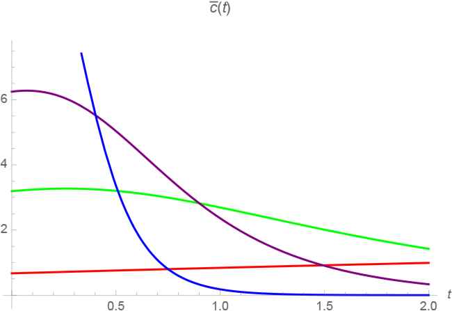
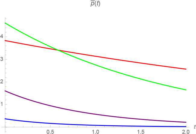
Graphical representations of the solutions. In order to explain the physical interpretation of solution surfaces in the analytical solutions, the two dimensional plots are shown below. The time variation of variables for the stock environmental asset function s(t), the consumption function c(t), and the costate variable p(t) are represented.

Figures 1–2–3 show the state, control and costate variable versus the time t, for the parametric choices φ, σ, ρ, m such that 0.9, 1.5, 2 and 3 with the same value integration constants c₁ and c₂.

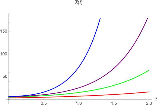
The use of transversality condition. The transversality condition for (3.33)–(3.35) reads

limt→∞e−ρtp¯(t)s¯(t)=e−mt(1+ϕ)(σ−1)+c2(1+ϕ)(σ−1)σ+tρ(1+σ)σ×(1+ϕ)σ(ρ+m(1+ϕ)(σ−1))−2σσσ(ρ+m(1+ϕ)(σ−1)−c1et(ρ+m(σ−1)(1+ϕ))σ)σ.(3.36)

which goes to zero if m(1+ϕ)(σ−1)+c2(1+ϕ)(σ−1)σ+ρ(1+σ)σ>0 and the use of the initial conditions for this case gives c₁ = 0.

The solution of initial-value-problem. Thus, the associated solution of the initial-value problem satisfying the transversality condition can be written as

s¯(t)=s¯0et(m−ρ+mϕ)σ(1+ϕ),c¯(t)=c¯0et(m−ρ+mϕ)σ(1+ϕ),p¯(t)=p¯0et(ϕρ+m(1+ϕ)(ϕ(σ−1)+σ))σ(1+ϕ).(3.37)

As a result, the growth rates for the control problem (3.1) and (3.1) defined by all of the economic variables are introduced by the following ratios

s¯˙s¯=m(ϕ+1)−ρσ(1+ϕ),(3.38)

c¯˙c¯=m(ϕ+1)−ρσ(1+ϕ),(3.39)

p¯˙p¯=ϕρ+m(1+ϕ)(ϕ(σ−1)+σ)σ(1+ϕ).(3.40)

3.3. Lagrangian approach

In addition, the equivalent second-order differential equation in terms of s(t) stock environmental asset variable can be constructed by implementing Euler-Lagrange differential operator to the Lagrangian according to the relation L=ps˙−H for the current value Hamiltonian (3.3) in the form

σs¨s+σϕs˙2+ss˙(ρ−m(1+σ)(1+ϕ))+m(m−ρ+mϕ)s2=0.(3.41)

Proposition 3.3.

The second-order nonlinear ordinary differential equation (3.41) possesses eight-dimensional Lie algebra L₈.

Proof.

The differential equation (3.41) yields the eight-dimensional symmetries L₈ as below

X1=∂∂t, X2=s∂∂s,X3=e(1+ϕ)mts−ϕ∂∂s, X4=e(mϕ+m−ρ)tσs−ϕ∂∂s,X5=s1+ϕme−(mϕ+m−ρ)tσ∂∂t+e−(mϕ+m−ρ)tσs2+ϕ∂∂s,X6=σs−1+ϕ(1+ϕ)mϕ+m−ρe−1(1+ϕ)mt∂∂t+e−1(1+ϕ)mts2+ϕ∂∂s,X7=1me(mϕσ−mϕ+mσ−m+ρ)tσ∂∂t+se(mϕσ−mϕ+mσ−m+ρ)tσ∂∂s,X8=σ(1+ϕ)mϕ+m−ρe−(mϕσ−mϕ+mσ−m+ρ)tσ∂∂t+se−(mϕσ−mϕ+mσ−m+ρ)tσ∂∂s.(3.42)

Remark 3.3.

If the second order ODE in the form x¨=ϕ possesses infinitesimals such that ξ(t,x), η (t,x), and its Lie point symmetry generator can be written as X = ξ∂_t +η∂_x, then the characteristic of X can be determined with O¸=η−ξx˙ [27–29]. Let A=∂t+x˙∂x+ϕ(t,x,x˙)∂x˙ denote the vector field of given equation; then the pair (∂_x, λ) where λ=−A(O¸)O¸ is a λ-symmetry associated to Lie point symmety X.

Remark 3.4.

If it is known that the pair (∂_x,λ) is a λ-symmetry of a given second order ODE, then first integral and integrating factor can be evaluated using the following procedure [28]:

1.
Derive a first integral ω(t,x,x˙) of first λ-prolongation υ[^λ,^(1)], that is a particular solution of the equation
ωx+λ⋅ωx˙=0,(3.43)
2.
Determine A(ω) and express A(ω) in terms of (t,ω) as A(ω)= F(t,ω).
3.
Find a first integral G of ∂_t + F(t,ω)∂_ω.
4.
Evaluate the final form of first integral as
I(t,x,x˙)=G(t,ω(t,x,x˙).(3.44)

Here, by using these symmetries, the first integrals of the equation can be evaluated with respect to the Jacobi and λ-symmetry approaches as two different cases.

Case I. In order to consider the λ-symmetry method, first, it can be shown that, for example, the symmetry X₃ leads to ξ= 0 and η= e^(1+φ)mts−^φ. Then via Remark 3.3, the characteristic function and the infinitesimal vector field are written by

O¸=e(1+ϕ)mts−ϕ, A=e(1+ϕ)mts−1−ϕ(ms(1+ϕ)−ϕs˙).(3.45)

Hence, the λ-symmetry is derived by in the form

λ3=m+mϕ−ϕs˙s.(3.46)

If the steps, which are expressed in Remark 3.4, are followed for λ-symmetry (3.46) and then the integration factor and first integral

μ3=e−(mϕ+m−ρ)tσsϕ,I3=−e−(mϕ+m−ρ)tσsϕ(ms−s˙),(3.47)

are found, respectively and the solution from the first integral I₃

s3(t)=e(mϕ+m−ρ)tσ(1+ϕ)(ρ+m(1+ϕ)(σ−1))−11+ϕ(−c1σ(1+ϕ)),(3.48)

is obtained, where c₁ is a constant. The corresponding λ-symmetries and integrating factors to vector fields X₁,...,X₈ are respectively,

λ1=−m2s2(1+ϕ)−s˙(sρ+σϕs˙)+ms(ρs+s˙(1+σ)(1+ϕ))σss˙,λ2=s˙s, μ2=s(ms−s˙)(−sρ+ms(1+ϕ)−s˙σ(1+ϕ)),λ3=m+mϕ−ϕs˙s, μ3=e−(mϕ+m−ρ)tσsϕ,λ4=−ρs−σϕs˙+ms(1+ϕ)σs, μ4=e−mt(1+ϕ)sϕ,λ5=λ2, μ5=μ2, λ6=λ2, μ6=μ2λ7=λ3, μ7=μ3, λ8=λ4, μ8=μ4. (3.49)

Case II. The possible Jacobi Last Multipliers are the reciprocals of the nonzero determinants of the possible matrices of (2.21). JLM_ij is indicated a multiplier, where the i and j refer to the symmetries used in the determinants. For example, by using the two symmetries, X₁ and X₂, one can write the corresponding determinant

Δ12=det[1s˙−m2s2(1+ϕ)−s˙(sρ+s˙σϕ)+ms(ρs+s˙(1+σ)(1+ϕ)sσ1000ss˙]=−σ(ms−s˙)(−ρs+ms(1+ϕ)−σs˙(1+ϕ)),

and then the Jacobi last multiplier JLM₁₂ is obtained as JLM12=1Δ12. Many different Jacobi last multiplier of the equation (3.41) can be generated via Lie symmetries (3.42), but we give some of them in the following

JLM12^=σ(s˙−ms)(−ρs+ms(1+ϕ)−s˙σ(1+ϕ)),JLM^17=et(ρ+m(1−σ)(1+ϕ))σmσ(s˙−ms)2(ρ−m(1+ϕ)),JLM^24=et(ρ−m−mϕ)σsϕσ−sρ+ms(1+ϕ)−s˙σ(1+ϕ),JLM^35=−et(ρ+m(1−σ)(1+ϕ))σm(s˙−ms)2(1+ϕ),JLM^58=emt(1+ϕ)ms−ϕσ(m−ρ+mϕ)(ms−s˙)(sρ−ms(1+ϕ)+s˙(1+ϕ))2,JLM^78=mσ(ρ−m−mϕ)(ms−s˙)(ρ+m(σ−1)(1+ϕ))(−sρ+ms(1+ϕ)−s˙σ(1+ϕ)),(3.50)

we use the JLM^ notation to denote the multipliers of the equation (3.41). Any ratio of two multipliers gives the first integral

I^=JLM^35JLM^78=e(ρ+m(1−σ)(1+ϕ))tσ(ρ+m(σ−1)(1+ϕ)(−ρs+ms(1+ϕ)−σ(1+ϕ)s˙)σ(1+ϕ)(ms−s˙)(mϕ+m−ρ),(3.51)

yielding the solution

s^(t)=e(mϕ+m−ρ)t+σln[ρ+c1e(ρ+m(σ−1)(1+ϕ)tσρ−m(1+c1e(ρ+m(σ−1)(1+ϕ))tσ−σ)(1+ϕ)]σ(1+ϕ)c2,(3.52)

where c₁ and c₂ are constants.

4. Planner’s Problem

As the last optimal control problem of the current study to analyze, we take into consideration the planner’s problem that defines a growth model in economics [22]. In the literature, this problem is analyzed numerically by using Runge-Kutta scheme based on exponential Lawson integration for nearly Hamiltonian systems [11]. In fact, this problem states that an economy produces a consumption good whose output is u(t), and the main purpose is to determine u(t) >0 that maximizes the integral

Max∫0∞e−ρt(ln(u)−λu2−bx)dt,(4.1)

subject to

x˙=u2−mx,(4.2)

where m > 0 is its natural rate of decay, x(t) is the stock of pollution, λand b are given positive constants, and ρis the discount factor for ρ >0. The initial and transversality conditions give

x(0)=x0, limt→∞e−ρtp(t)x(t)=0,(4.3)

and then the current value Hamiltonian for (4.1) is written via (2.8) in the form

H=ln(u)−λu2−bx+p(u2−mx),(4.4)

where p(t) is the costate variable. FOCs for the system (2.12)–(2.12) are

p=2λu2−12u2,(4.5)

x˙=u2−mx,(4.6)

p˙=b+mp+ρp.(4.7)

Similarly, if we focus on the present value Hamiltonian function including the discount factor of the form

H¯=e−ρt(ln(u¯)−λu¯2−bx¯)+p¯(u¯2−mx¯),(4.8)

and then the corresponding FOCs, which are Hamiltonian equations, via equations (2.9)–(2.11)

p¯=e−ρt(2λu¯2−1)2u¯2,(4.9)

x¯˙=u¯2−mx¯,(4.10)

p¯˙=e−ρtb+mp¯,(4.11)

are derived. The system of equations (4.5)–(4.7) and (4.9)–(4.11), in fact, do not define a coupled system of differential equations as opposed to the previous cases. However, both equations (4.5)–(4.7) and (4.9)–(4.11) can be rewritten as a single equation in terms of variable x(t) by eliminating variables p(t) and u(t) such that

x¨−2(b+λ(m+ρ))(mx+x˙)2+(2m+ρ)x˙+m(m+ρ)x=0.(4.12)

By the use of the relationship between Lagrangian and Hamiltonian (present value Hamiltonian), the Lagrangian function related to Hamiltonian function (4.8) of the differential equation (4.12)

L¯=e−ρt(−ln(mx+x˙)+bx+λ(mx+x˙)),(4.13)

is written. It can also be checked that if the Euler-Lagrange operator is applied to (4.13) and then the same equation with the equation in (4.12) is achieved. It is a fact that such equation is a second-order ODE admitting a two-dimensional symmetry algebra and it could therefore be integrated by quadratures by the classical Lie method. The same applies to equation (3.41), which admits an eight-dimensional symmetry algebra. However, we deal with λ-symmetry approach by considering the relation the Lie point symmetries to obtain an analytic solution to the for economic growth considered in this study.

Proposition 4.1.

The second-order nonlinear ordinary differential equation (4.12) has two-dimensional Lie algebra L₂.

Proof.

It can be easily checked that the equation (4.12) possesses two-dimensional Lie symmetries from solutions of the corresponding determining equations, namely,

X1=∂∂t, X2=e−mt∂∂x.(4.14)

Based on the procedure given by Remark 3.3 and Remark 3.4, the generator X₂ yields

O¸=e−mt, A=−me−mt, λ1=−m,(4.15)

and the integration factor and the first integral of the equation (4.12)

μ=1(mx+mx˙)(m(−1+2(mx+x˙)λ)−ρ+2(mx+x˙)(b+λρ)),(4.16)

I1=−t+1m+ρln[−m+2b(mx+x˙)+2m(mx+x˙)λ−ρ+2(mx+x˙)λρmx+x˙],(4.17)

are found.

Analytical solutions. The first integral I₁ gives the solution for the stock of pollution variable

x(t)=e−mtc2+(m+ρ)Hypergeometric2F1[1,mm+ρ,2m+ρm+ρ,e(c1+t)(m+ρ)2(b+λ(m+ρ))]2m(b+λ(m+ρ)),(4.18)

which involves an hypergeometric function, where c₁ and c₂ are constants. In addition, by using (4.5)–(4.7) the other solutions for the variables u(t) and p(t)

u(t)=m+ρ2b−e(c1+t)(m+ρ)+2λ(m+ρ),(4.19)

p(t)=e(c1+t)(m+ρ)−2b2(m+ρ),(4.20)

are determined.

Remark 4.1.

There may exist JLMs not derived from symmetries via (2.21). Therefore, although equation (4.12) has only two Lie point symmetries, the JLM method could still be applicable to obtain first integrals of the equation.

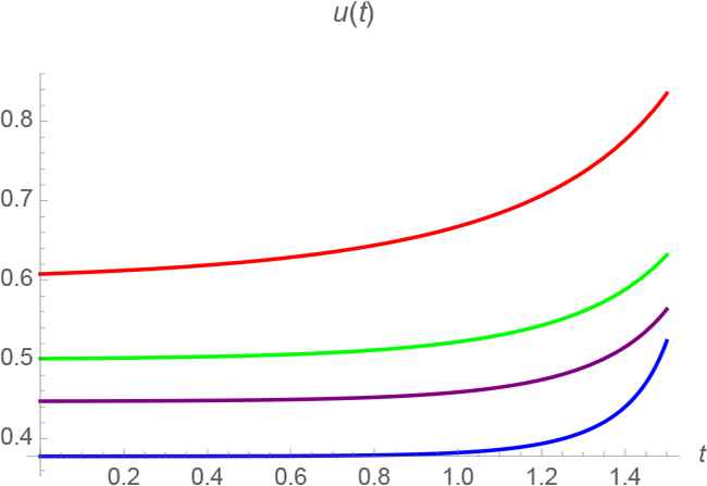
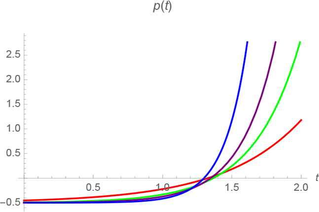
Graphical representations of the solutions. Similarly, in order to explain the physical interpretation of solution surfaces in the analytical solutions, the two dimensional plots are shown below. The time variation of variables for the consumption good output function u(t), stock of pollution x(t), and the costate variable p(t) are represented.

Figures 4–5–6 represent the state, control and costate variables of planner’s problem (4.1) versus the time t, with the values of the parameters λ, b, ρand m are chosen by 0.9, 1.5, 2 and 3 for the same value integration constants c₁ and c₂.

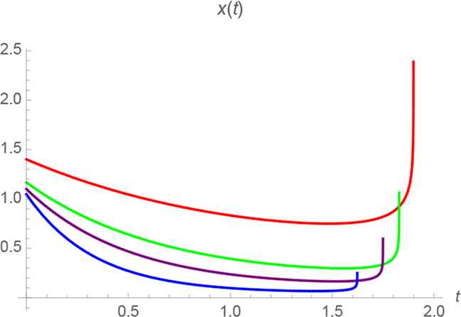
The use of transversality condition. On the other hand, the transversality condition (4.3) by considering the equations (4.18)–(4.20) requires that ρ >0. Thus, the growth rates are

x˙x=−m,(4.21)

u˙u=−12(m+ρ),(4.22)

for b = −λ (m + ρ). And finally, using the condition c₁ = 0, we have

p˙p=m+ρ,(4.23)

which points out that the growth rate for the costate variable p gets the value m + ρas t → ∞.

Remark 4.2.

The relations x=x¯ and u=u¯ exist here since we have only one equation corresponding to the current and present value Hamiltonians. Hence, the relations p=p¯ert and H=H¯ert are hold.

Proposition 4.2.

It is possible to obtain the similar results given by (4.18)–(4.19) for the model (4.1) and (4.2) by using the partial Hamiltonian method.

Proof.

The partial Hamiltonian method can also be applied to the maximization problem given in (4.1) and (4.2) by the current value Hamiltonian (4.4). We here only represent the results based on this method for the problem (4.1) and (4.2). The corresponding infinitesimal functions and the gauge function B [32] are found as

ξ=0, η=e−t(m+ρ)c1(m+ρ)(m+ρ)(b+λ(m+ρ)), B=c2−be−t(m+ρ)c1(m+ρ)(b+λ(m+ρ)),(4.24)

where c₁ and c₂ are constants. By using the relation I = pη− ξ H − B, first integral in terms of costate variable p(t)

I2=e−t(m+ρ)(b+p(m+ρ))(m+ρ)(b+λ(m+ρ)).(4.25)

can be written. Hence, the solution for the costate variable obtained from the relation I₂ = c₃, where c₃ is constant, takes the form

p(t)=c3et(m+ρ)λ(m+ρ)2+b(−1+c3et(m+ρ)(m+ρ))m+ρ.(4.26)

On the other hand, it can be checked that if the FOCs are used to determine the solution of stock of pollution x(t) then the necessary calculations confirm that the same solution is found with the solution given in (4.18).

Remark 4.3.

For all first integrals I and Ī obtained in three different economic models, it can be verified that the relations DI = 0 and DĪ = 0 yield the corresponding original differential equations.

5. Conclusions and Remarks

In this study, we analyze for the first time in the literature the analytical solutions of some economical models, which are entitled the optimal control model with environmental asset and the planner’s problem, by using different mathematical approaches having notable mathematical connections based on the symmetry group theory. In the literature, the optimal control problems in economic growth theory are generally investigated by numerical methods because of complexity of the formulizations of the models. The methods used here focus to determine analytical solutions of the optimal control problems in the theory of economics and it can be seen as one of the remarkable contributions in this study. Besides, another considerable property of the study is based on the fact that the first-order conditions (FOCs) are considered not only for the current value Hamiltonian but also for the present value Hamiltonian. The first-order conditions are called Hamiltonian equations for the case of present value Hamiltonians.

The novel and nontrivial analytical solutions for the present value Hamiltonians are investigated. Additionally, the initial-value problems are studied for the cases of optimal control model with environmental asset and the planner’s problems. After obtaining the analytical solutions, the corresponding initial conditions are applied and the solution for the related initial-value problem is determined. In addition to the initial-values related problems, the transversality conditions, which are optimal conditions often used to characterize the optimal paths of economic models, are also considered for the solution of the models. The growth rates for the control problem defined by all economic variables are introduced by the ratios of the variables and their time derivatives.

As one of the mathematical approaches, the Jacobi last multiplier method connected to the Lie symmetry groups is also applied for investigating new first integrals (conservation forms) for the system of first-order differential equations. It is shown that any ratio of two different multipliers MM˜ represents a first integral of the associated system. In this analysis, the noteworthy relation between the Lie point symmetries and Jacobi last multiplier approach based on obtaining solutions of the economic models is represented for the economic models in this study. In addition, λ-symmetry approach is considered by transforming the system of first-order differential equations to an equivalent single second-order ordinary differential equation. By using the relation between Lie point symmetries and λ-symmetries, the associated new first integral, integration factor and analytical solution are obtained.

For the optimal control model with environmental asset, we show that system of first-order differential equations associated with the current value Hamiltonian and the present value Hamiltonian have different forms and this property is an important reason to deal with two different Hamiltonian functions based on the analytical solutions for the optimal control problems. We also prove a remarkable distinction between the current Hamiltonian and the present Hamiltonian functions with respect to their Lie point symmetries. In the case of the optimal growth model with environmental asset we have four-dimensional Lie algebra L₄ for the current value Hamiltonian and five-dimensional Lie algebra L₆ for the present vale Hamiltonian. This can be seen as an important property for the analysis of the optimal control problems.

For the analysis of the first-order system of ordinary differential equations, we indicate that the first integrals are algebraic equations of the dependent variables since the system has only first-order derivatives. However, in the case of single second-order ordinary differential equations, the first integrals involve the first-order time derivatives of the unknown functions as can be expected. For the optimal growth model with environmental asset, we obtain not only the analytical solutions but also the solutions of the initial-value problem based on the initial conditions and the transversality condition. For the planner’s problem, we also show that the relations x=x¯ and u=u¯ exist and one can have the same equation corresponding to the current and present value Hamiltonians. Therefore, the relations p=p¯ert and H=H¯ert are valid for the planner’s problem.

In this study, we also emphasize the fact that the applied procedures such as JLM and λ-symmetries and connection with Lie symmetries can represent new perspectives for the optimal control problems in economic growth models. For example, the method of Jacobi can provide the first integrals for a given equation since any ratio of two multipliers equal to a first integral and then the growth rates of optimal growth model with environmental asset can be determined for the results of current and present value Hamiltonians. Additionally, the analytical solutions for the different value of the parameters are represented by the solution graphs and some mathematical economic comments belong to them are explained. In addition, to compare the results for the case of the planner’s optimal control model, we prove that the application of the mathematical methods considered in the study and the partial Hamiltonian method yield the same results.

In addition, from another mathematical point of view, it is known that it is not possible to apply the phase diagram approach as the usual method since the equilibria can not be defined well for analysis of the optimal control problems including the independent time exponential term that the present value Hamiltonian function involves. In this study, however, we represent that the analysis of optimal control problems in economic growth models by the theory of Lie groups involving not only the current value Hamiltonian function but also present value Hamiltonian function can be carried out analytically and effectively.

References

[1]D. Acemoglu, Introduction to modern economic growth, Department of Economics, UCLA, 2007. Levine’s Bibliography

[2]S.S. Akhiev and T. Özer, Symmetry groups of the equations with nonlocal structure and an application for the collisionless Boltzmann equation, Int. J. Eng. Sci, Vol. 43, No. 1–2, 2005, pp. 121-137.

[3]K.J. Arrow and M. Kurz, Public investment, the rate of return and optimal fiscal policy, Johns Hopkins Press, Baltimore-London, 1970.

[4]R.J. Barro and X. Sala-i-Martin, Economic growth, The MIT press, Cambridge, 2004.

[5]G. Bauman, Symmetry analysis of differential equations using MathLie, Springer-Verlag, New York, 2000.

[6]R. Bellman, Dynamic programming, 1st edition, Princeton University Press, Princeton, NJ, USA, 1957.

[7]L. Bianchi, Lezioni sulla Teoria dei Gruppi Continui Finiti di Trasformazioni, Enrico Spoerri, Pisa, 1918.

[8]G.W. Bluman and S. Kumei, Symmetries and Differential Equations, Springer-Verlag, New York, 1989.

[9]D. Cass, Optimum growth in an aggregative model of capital accumulation, Review of Economic Studies, Vol. 32, No. 3, 1965, pp. 233-240.

[10]A. Cheviakov, GeM software package for computation of symmetries and conservation laws of differential equations, Comp. Phys. Comm, Vol. 176, 2007, pp. 48-61.

[11]F. Diele, C. Marangi, and S. Ragni, Exponential Lawson integration for nearly Hamiltonian systems arising in optimal control, Mathematics and Comp. in Sim, Vol. 81, 2011, pp. 1057-1067.

[12]R. Dorfman, An economic interpretation of optimal control theory, The American Economic Review, Vol. 59, No. 5, 1969, pp. 817-831.

[13]O. Esen and P. Guha, On time-dependent Hamiltonian realizations of planar and nonplanar systems, Journal of Geometry and Physics, Vol. 127, 2018, pp. 32-45.

[14]G. Gaeta and P. Morando, PDEs reduction and λ-symmetries, Note Di Matematica, Vol. 23, No. 2, 2004/2005, pp. 33-73.

[15]G. Gaeta, Lambda and µ-symmetries, Symmetry and Perturbation Theory, World Scientific, 2005, pp. 99-105.

[16]G. Gün Polat and T. Özer, First integrals, integrating factors and invariant solutions of the path equation based on Noether and λ-symmetries, Abstract and Applied Analysis, 2013. Article ID 284653

[17]G. Gün Polat and T. Özer, On analysis of nonlinear dynamical systems via methods connected with λ-symmetry, Nonlinear Dyn, Vol. 85, No. 3, 2016, pp. 1571-1595.

[18]G. Gün Polat and T. Özer, New conservation laws, Lagrangian forms and exact solutions of modified-Emden equation, J. Comput. Nonlinear Dynam, Vol. 12, No. 4, 2017, pp. 041001.

[19]C.G.J. Jacobi, Sul principio dellultimo moltiplicatore, e suo come nuovo principio generale di meccanica, Giornale Arcadico di Scienze Lettere ed Arti, Vol. 99, 1844, pp. 29-146.

[20]C.G.J. Jacobi, Theoria novi multiplicatoris systemati aequationum differentialium vulgarium applicandi, J. Reine Angrew. Math. (Crelle J.), Vol. 27, 1844, pp. 199-268.

[21]A.A. LeKama and K. Schubert, A note on the consequences of an endogenous discounting depending on the environmental quality, Macroecon. Dyn, Vol. 11, No. 2, 2007, pp. 272-289.

[22]D. Leonard and N. Van Long, Optimal Control Theory and Static Optimization in Economics, Cambridge Universtiy Press, 1992.

[23]S. Lie, Vorlesungen über Differentialgleichungen mit bekannten infinitesimalen Transformationen, Teubner, Leipzig, 1912.

[24]S. Lie, Veralgemeinerung und neue Verwerthung der Jacobischen Multiplicator-Theorie, Fordhandlinger i Videnokabs-Selshabet i Christiania, 1874, pp. 255-274.

[25]R. Lucas, On the Mechanics of Economic Development, Journal of Monetary Economics, Vol. 22, No. 1, 1988, pp. 3-42.

[26]R. Mohanasubha, V.K. Chandrasekar, M. Senthilvelan, and M. Lakshmanan, Interplay of symmetries, null forms, Darbou polynomials, integrating factors and Jacobi multipliers in integrable second order differential equations, Proc. R. Soc. A, Vol. 470, 2014.

[27]C. Muriel and J.L. Romero, New methods of reduction for ordinary differential equations, IMA J. Appl. Math, Vol. 66, No. 2, 2001, pp. 111-125.

[28]C. Muriel and J.L. Romero, First integrals, integrating factors and symmetries of second order differential equations, J. Phys. A: Math. Theor, Vol. 42, No. 36, 2009.

[29]C. Muriel, J.L. Romero, and A. Ruiz, λ-Symmetries and integrability by quadratures, IMA Journal of App. Math, Vol. 82, No. 5, 2017, pp. 1061-1087.

[30]R. Naz, F.M. Mahomed, and A. Chaudhry, A partial Lagrangian method for dynamical systems, Nonlinear Dyn, Vol. 84, No. 3, 2016, pp. 1783-1794.

[31]R. Naz, The applications of the partial Hamiltonian approach to mechanics and other areas, Int. J. Non. Linear Mech, Vol. 86, No. 1, 2016, pp. 1-6.

[32]R. Naz, F.M. Mahomed, and A. Chaudhry, A partial Hamiltonian approach for current value Hamiltonian systems, Commun. Nonlinear Sci. Numer. Simul, Vol. 19, No. 10, 2014, pp. 3600-3610.

[33]R. Naz, F.M. Mahomed, and A. Chaudhry, Closed-form solutions for the Lucas-Uzawa model of economic growth via the partial Hamiltonian approach, Commun. Nonlinear Sci. Numer. Simul, Vol. 30, No. 1–3, 2016, pp. 299-306.

[34]M.C. Nucci, Jacobi Last Multiplier and Lie symmetries: A Novel Application of an Old Relationship, J. Nonlinear Math. Phys, Vol. 12, No. 2, 2005, pp. 284-304.

[35]M.C. Nucci, Seeking (and Finding) Lagrangians, Theoretical and Mathematical Physics, Vol. 160, No. 1, 2009, pp. 1014-1021.

[36]M.C. Nucci and P.G.L. Leach, Lagrangians Galore, J. Math. Phys., Vol. 48 123510, No. 12, 2007.

[37]M.C. Nucci and P.G.L. Leach, An old method of Jacobi to find Lagrangians, J. Nonlinear Math. Phys, Vol. 16, No. 4, 2009, pp. 431-441.

[38]M.C. Nucci and K. M. Tamizhmani, Using an old method of Jacobi to derive Lagrangians: A nonlinear dynamical system with variable coefficients, Nuovo Cimente Della Societa Italiana Di Fisica B-Basic Topics in Physics, Vol. 125, No. 3, 2010, pp. 255-269.

[39]P.J. Olver, Applications of Lie Groups to Differential Equations, Springer-Verlag, New-York, 1993.

[40]Ö. Orhan and T. Özer, On µ-symmetries, µ-reductions and µ-conservation laws of Gardner equation, J. Nonlinear Math. Phys, Vol. 26, 2019, pp. 1-22.

[41]T. Özer, Symmetry group classification for two-dimensional elastodynamics problems in nonlocal elasticity, Int. J. Eng. Sci, Vol. 41, No. 18, 2003, pp. 2193-2211.

[42]F. Ramsey, A Mathematical theory of saving, Economic Journal, Vol. 38, 1928, pp. 543-559.

[43]P.M. Romer, The origins of endogenous growth, The Journal of Economic Perspectives, Vol. 8, No. 1, 1994, pp. 3-22.

[44]A. Ruiz and C. Muriel, On the integrability of Liénard I-type equations via λ-symmetries and solvable structures, Applied Math. Comp, Vol. 339, 2018, pp. 888-898.

[45]R. Solow, A contribution to the theory of economic growth, The Quarterly Journal of Economics, Vol. 70, No. 1, 1956, pp. 65-94.

[46]H. Uzawa, Optimum Technical Change in An Aggregative Model of Economic Growth, International Economic Review, 1965.

<Previous Article In Issue

Download article (PDF)

Next Article In Issue>

Journal: Journal of Nonlinear Mathematical Physics
Volume-Issue: 27 - 1
Pages: 106 - 129
Publication Date: 2019/10/25
ISSN (Online): 1776-0852
ISSN (Print): 1402-9251
DOI: 10.1080/14029251.2020.1683985 How to use a DOI?
Open Access: This is an open access article distributed under the CC BY-NC 4.0 license (http://creativecommons.org/licenses/by-nc/4.0/).

Cite this article

ris enw bib

TY  - JOUR
AU  - Gülden Gün Polat
AU  - Teoman Özer
PY  - 2019
DA  - 2019/10/25
TI  - The Group-Theoretical Analysis of Nonlinear Optimal Control Problems with Hamiltonian Formalism
JO  - Journal of Nonlinear Mathematical Physics
SP  - 106
EP  - 129
VL  - 27
IS  - 1
SN  - 1776-0852
UR  - https://doi.org/10.1080/14029251.2020.1683985
DO  - 10.1080/14029251.2020.1683985
ID  - Polat2019
ER  -

download .riscopy to clipboard