
Multicomplex solitons
- DOI
- 10.1080/14029251.2020.1683963How to use a DOI?
- Keywords
- nonlinear wave equations; solitons; quaternions; coquaternions; octonions
- Abstract
We discuss integrable extensions of real nonlinear wave equations with multi-soliton solutions, to their bicomplex, quaternionic, coquaternionic and octonionic versions. In particular, we investigate these variants for the local and nonlocal Korteweg-de Vries equation and elaborate on how multi-soliton solutions with various types of novel qualitative behaviour can be constructed. Corresponding to the different multicomplex units in these extensions, real, hyperbolic or imaginary, the wave equations and their solutions exhibit multiple versions of antilinear or 𝒫𝒯-symmetries. Utilizing these symmetries forces certain components of the conserved quantities to vanish, so that one may enforce them to be real. We find that symmetrizing the noncommutative equations is equivalent to imposing a 𝒫𝒯-symmetry for a newly defined imaginary unit from combinations of imaginary and hyperbolic units in the canonical representation.
- Copyright
- © 2020 The Authors. Published by Atlantis and Taylor & Francis
- Open Access
- This is an open access article distributed under the CC BY-NC 4.0 license (http://creativecommons.org/licenses/by-nc/4.0/).
1. Introduction
The underlying mathematical structure of quantum mechanics, a Hilbert space over the field of complex numbers, can be generalized and modified in various different ways. One may for instance re-define the inner product of the Hilbert space or alter, typically enlarge, the field over which this space is defined. The first approach has been pursued successfully since around twenty years [8], when it was first realized that the modification of the inner product allows to include non-Hermitian Hamiltonians into the framework of a quantum mechanical theory. When these non-Hermitian Hamiltonians are 𝒫𝒯-symmetric/quasi-Hermitian [7, 28, 32] they possess real eigenvalues when their eigenfunctions are also 𝒫𝒯-symmetric or pairs of complex conjugate eigenvalues when the latter is not the case. The reality of the spectrum might only hold in some domain of the coupling constant, but break down at what is usually referred to as an exceptional point when at least two eigenvalues coalesce. Higher order exceptional points may occur for larger degeneracies. In order to unravel the structure of the neighbourhood of these points one can make use of the second possibility of generalizations of standard quantum mechanics and change the type of fields over which the Hilbert space is defined. This view helps to understand the bifurcation structure at these points and has been recently investigated for the analytically continued Gross-Pitaevskii equation with bicomplex interaction terms [16, 18, 21]. In a similar spirit, systems with finite dimensional Hilbert spaces have been formulated over Galois fields [37]. Hyperbolic extensions of the complex Hilbert space have been studied in [38]. The standard Schrödinger equation was bicomplexified in [3] and further studied in [4–6, 35]. Quaternionic and coquaternionic quantum mechanics and quantum field theory have been studied for a long time, see e.g. [2, 19, 20], mainly motivated by the fact that they may be related to various groups and algebras that play a central role in physics, such as SO(3), the Lorentz group, the Clifford algebra or the conformal group. Recently it was suggested that they [9] provide a unifying framework for complexified classical and quantum mechanics. Octonionic Hilbert spaces have been utilized for instance in the study of quark structures [22].
Drawing on various relations between the quantum mechanical setting and classical integrable nonlinear systems that possess soliton solutions, such as the formal identification of the L operator in a Lax pair as a Hamiltonian, many of the above possibilities can also been explored in the latter context. Most direct are the analogues of the field extensions. Previously we demonstrated [12, 13] that one may consistently extend real classical integrable nonlinear systems to the complex domain by maintaining the reality of the energy. Here we go further and investigate multicomplex versions of these type of nonlinear equations. We demonstrate how these equations can be solved in several multicomplex settings and study some of the properties of the solutions. We explore three different possibilities to construct solutions that are not available in a real setting, i) using multicomplex shifts in a real solutions, ii) exploiting the complex representations by defining a new imaginary unit in terms of multicomplex ones and iii) exploiting the idempotent representation. We take 𝒫𝒯-symmetry as a guiding principle to select out physically meaningful solutions with real conserved quantities, notably real energies. We clarify the roles played by the different types of 𝒫𝒯-symmetries. For the noncommutative versions, that is quaternionic, coquaternionic and octonionic, we find that imposing certain 𝒫𝒯-symmetries corresponds to symmetrizing the noncommutative terms in the nonlinear differential equations.
Our manuscript is organized as follows: In section 2 we discuss the construction of bicomplex multi-solitons for the standard Korteweg de-Vries (KdV) equation and its nonlocal variant. We present two different types of construction schemes leading to solutions with different types of 𝒫𝒯-symmetries. We demonstrate that the conserved quantities constructed from these solutions, in particular the energy, are real. In section 3, 4 and 5 we discuss solution procedures for noncommutative versions of the KdV equation in quaternionic, coquaternionic and octonionic form, respectively. Our conclusions are stated in section 6.
2. Bicomplex solitons
2.1. Bicomplex numbers and functions
We start by briefly recalling some key properties of bicomplex numbers and functions to settle our notations and conventions. Denoting the field of complex numbers with imaginary unit ı as
The canonical basis is spanned by the units ℓ, ı, 𝚥, k, involving the two imaginary units ı and 𝚥 with ı2 = 𝚥2 = −1, so that the representations in equations (2.2) and (2.3) naturally prompt the notion to view these numbers as a doubling of the complex numbers. The real unit ℓ and the hyperbolic unit k = ı𝚥 square to 1, ℓ2 = k2 = 1. The multiplication of these units is commutative with further products in the Cayley multiplication table being ℓı = ı, ℓ 𝚥 = 𝚥, ℓk = k, ık = −𝚥, 𝚥k = −ı. The idempotent representation (2.5) is an orthogonal decomposition obtained by using the orthogonal idempotents
Arithmetic operations are most elegantly and efficiently carried out in the idempotent representation (2.5). For the composition of two arbitrary numbers na and nb we have
The hyperbolic numbers (or split-complex numbers) 𝔻 = {a1ℓ + a4k | a1, a4 ∈ ℝ} are an important special case of 𝔹 obtained in the absence of the imaginary units ı and 𝚥, or when taking a2 = a3 = 0.
The same arithmetic rules as in (2.9) then apply to bicomplex functions. In what follows we are most interested in functions depending on two real variables x and t of the form f(x, t) = ℓp(x, t) + ıq(x, t) + 𝚥r(x, t) + ks(x, t) ∈ 𝔹 involving four real fields p(x, t), q(x, t), r(x, t), s(x, t) ∈ ℝ. Having kept the functional variables real, we also keep our differential real, so that we can differentiate f (x, t) componentwise as ∂x f(x, t) = ℓ∂x p(x, t) + ı∂xq(x, t) + 𝚥∂xr(x, t) + k∂xs(x, t) and similarly for ∂t f(x, t). For further properties of bicomplex numbers and functions, such as for instance computing norms, see for instance [17, 26, 29, 30].
2.2. 𝒫𝒯-symmetric bicomplex functions and conserved quantities
As there are two different imaginary units, there are three different types of conjugations for bicomplex numbers, corresponding to conjugating only ı, only 𝚥 or conjugating both ı and 𝚥 simultaneously. This is reflected in different symmetries that leave the Cayley multiplication table invariant. As a consequence we also have three different types of bicomplex 𝒫𝒯-symmetries, acting as
Decomposing a density function for any conserved quantity as
2.3. The bicomplex Korteweg-de Vries equation
Using the multiplication law (2.9) for bicomplex functions, the KdV equation for a bicomplex field in the canonical form
We recall that we keep here our space and time variables, x and t, to be both real so that also the corresponding derivatives ∂x and ∂t are not bicomplexified.
When acting on the component functions the 𝒫𝒯-symmetries (2.10)–(2.12) are implemented in (2.16) as
We observe that (2.16) allows for a scaling of space by the hyperbolic unit k as x → k x, leading to a new type of KdV-equation with u → h
Next we consider various solutions to these different versions of the bicomplex KdV-equation, discuss how they may be constructed and their key properties.
2.3.1. One-soliton solutions with broken 𝒫𝒯-symmetry
We start from the well known bright one-soliton solution of the real KdV equation (2.16)
Noting that the complex solution uiθ,α(x, t) studied in [13], can be expressed as uiθ,α(x, t) = pa,θ;α(x − a/α, t)+iqa,θ;α(x − a/α, t), we can also expand the bicomplex solution (2.25) in terms of the complex solution as
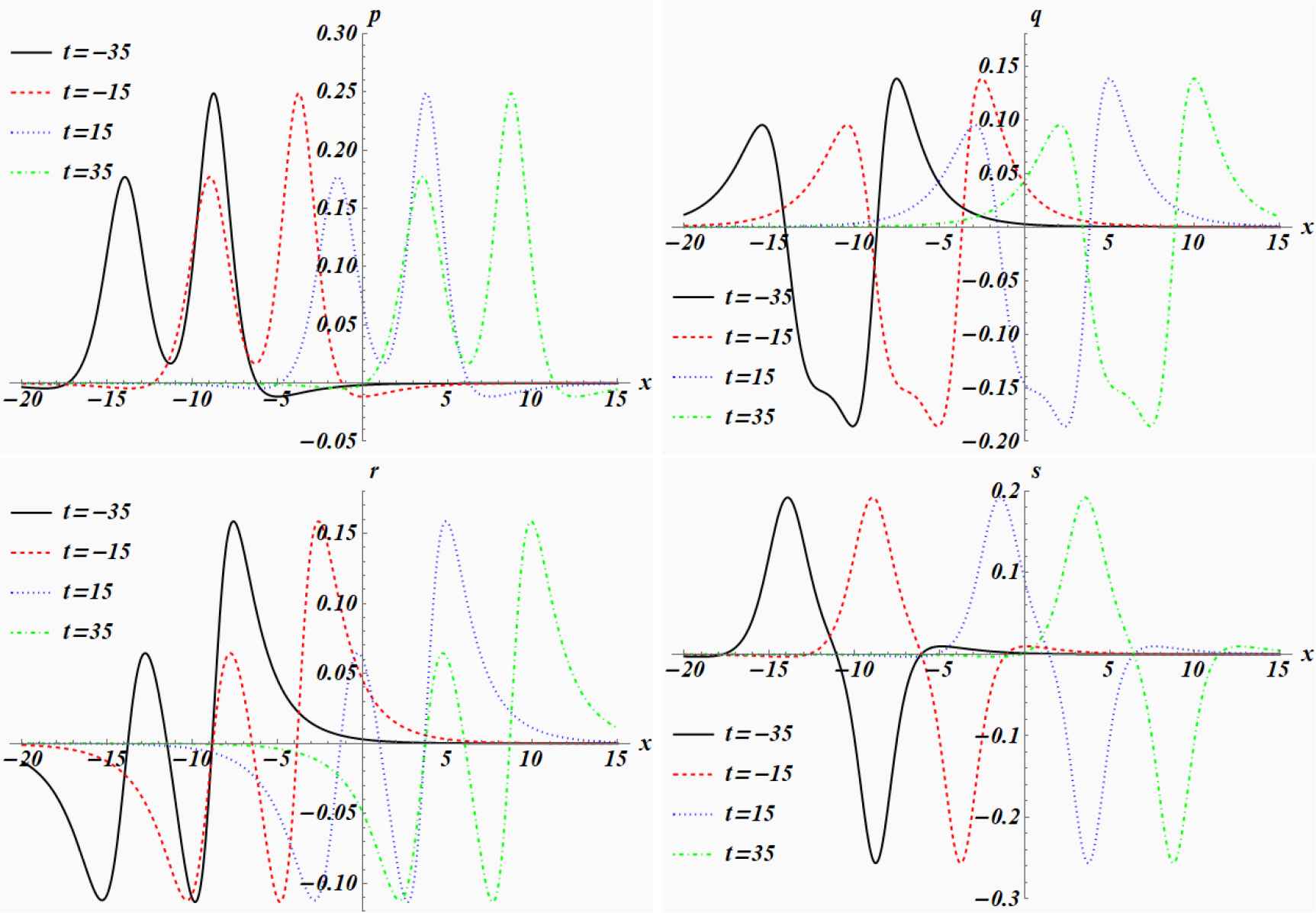
Canonical component functions p, q, r and s (clockwise starting in the top left corner) of the decomposed onesoliton solution uρ,θ,ϕ,χ;α to the bicomplex KdV equation (2.16) with broken 𝒫𝒯-symmetry at different times for α = 0.5, ρ = 1.3, θ = 0.4, ϕ = 2.0 and χ = 1.3.
In figure 2.3.1 we depict the canonical components of this solution at different times. We observe in all of them that the one-soliton solution is split into two separate one-soliton-like components moving parallel to each other with the same speed. The real p-component can be viewed as the sum of two bright solitons and the hyperbolic s-component is the sum of a bright and a dark soliton. This effect is the results of the decomposition of each of the components into a sum of the functions pa,b;α or qa,b;α, as defined in (2.26), at different values of a, b, but the same value of α. Since a and b control the amplitude and distance, whereas regulates the speed, the constituents travel at the same speed. We recall that this type of behaviour of degenerate solitons can neither be created from a real nor a complex two-soliton solution [11, 15]. So this is a novel type of phenomenon for solitons previously not observed.
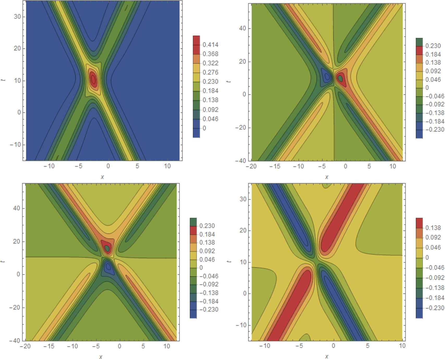
Head-on collision of a bright soliton with a dark soliton in the canonical components p, q, r, s (clockwise starting in the top left corner) for the one-soliton solution hρ,θ,ϕ,χ;α to the bicomplex KdV equation (2.16) with broken 𝒫𝒯-symmetry for α = 0.5, ρ = 1.3, θ = 0.1, ϕ = 2.0 and χ = 1.3. Time is running vertically, space horizontally and contours of the amplitudes are colour-coded indicated as in the legends.
In general, the solution (2.24) is not 𝒫𝒯-symmetric with regard to any of the possibilities defined above. It becomes 𝒫𝒯ı𝚥-symmetric when ρ = χ = 0, 𝒫𝒯ık-symmetric when ρ = χ = ϕ = 0 and 𝒫𝒯jk-symmetric when ρ = χ = θ = 0.
A solution to the new KdV equation (2.23) is constructed as
In figure 2.3.1 we depict the canonical component functions of this solution. We observe that the one-soliton solution is split into two one-soliton-like structures that scatter head-on with each other. The real p-component consists of a head-on scattering of two bright solitons and hyperbolic the s-component is a head-on collision of a bright and a dark soliton. Given that uρ,θ,ϕ,χ;α and hρ,θ,ϕ,χ;α(x, t) differ in the way that one of its constituent functions is time-reversed this is to be expected.
2.3.2. 𝒫𝒯ij-symmetric one-soliton solution
An interesting solution can be constructed when we start with a complex 𝒫𝒯ık and a complex 𝒫𝒯𝚥k symmetric solution to assemble the linear decomposition of an overall 𝒫𝒯ı𝚥-symmetric solution with different velocities. Taking in the decomposition (2.17) v(x, t) = uıθ,α(x, t) and w(x, t) = u𝚥ϕ,β(x, t), we can build the bicomplex KdV-solution in the idempotent representation
The expanded version in the canonical representation becomes in this case
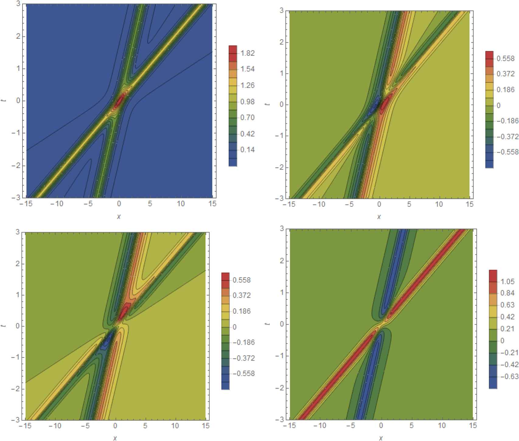
A fast bright soliton overtaking a slower bright soliton in the canonical component functions p, q, r and s (clockwise starting in the top left corner) for the one-soliton solution ûθ,ϕ;α,β to the bicomplex KdV equation (2.16) with 𝒫𝒯ij-symmetry for α = 2.1, β = 1.1, θ = 0.6 and ϕ = 1.75.
2.3.3. Multi-soliton solutions
The most compact way to express the N-soliton solution for the real KdV equation in the form (2.16) is
We could now take the shifts μ1, μ2, . . ., μn ∈ 𝔹 and expand (2.33) into its canonical components to obtain the N-soliton solution for the bicomplex equation. Alternatively we may also construct N-solitons in the idempotent basis in analogy to (2.32). We demonstrate here the latter approach for the two-soliton. From (2.33) we observe that the second derivative will not alter the linear bicomplex decomposition and it is therefore useful to introduce the quantity w(x, t) as u = wx. Thus a complex one-soliton solution can be obtained from
Noting that
Using (2.37) to define the two complex quantities
Then by construction uθ1,θ2,θ3,θ4,ϕ1,ϕ2,ϕ3,ϕ4;α1,α2,β1,β2 = (w2)x is a bicomplex two-soliton solution with four speed parameters. In a similar fashion we can proceed to construct N-soliton for N > 2.
2.3.4. Real and hyperbolic conserved quantities
Next we compute the first conserved quantities the mass m, the momentum p and the energy E, see e.g. [12, 13]
Decomposing the relevant densities into the canonical basis, u as in (2.15), u2 as
These values are the same as those found in [13] for the complex solitons. Given that the 𝒫𝒯-symmetries are all broken this is surprising at first sight. However, considering the representation (2.28) this is easily understood when using the result of [13]. Then m(uρ,θ,ϕ,χ;α) is simply ℓ/2(2α + 2α) + 𝚥/2(2α − 2α) = 2αℓ. We can argue similarly for the other conserved quantities.
For the 𝒫𝒯ij-symmetric solution ûθ,ϕ;α,β we obtain the following hyperbolic values for the conserved quantities
The values become real and coincide with the expressions (2.45)–(2.47) when we sum up the contributions from the real and hyperbolic component or in the degenerate case when we take the limit β → α.
2.4. The bicomplex Alice and Bob KdV equation
Various nonlocal versions of nonlinear wave equations that have been overlooked previously have attracted considerable attention recently. In reference to standard scenarios in quantum cryptography some of them are also often referred to as Alice and Bob systems. These variants of the nonlinear Schrödinger or Hirota equation [1, 10, 27, 33] arise from an alternative choice in the compatibility condition of the two AKNS-equations. For the KdV equation (2.16) they can be constructed [23–25] by choosing u(x, t) = 1/2[a(x, t) + b(x, t)], with the constraint 𝒫𝒯 a(x, t) = a(−x, −t) = b(x, t), thus converting it into an equation that can be decomposed into two equations, the Alice and Bob KdV (ABKdV) equation
In a similar way as the two AKNS-equations can be made compatible by a suitable transformation map, these two equations are converted into each other by a 𝒫𝒯-transformation, i.e. 𝒫𝒯 (2.51) ≡ (2.52). Evidently the decomposition is not unique and one may also add and subtract a constrained function of a and b or consider different types of maps to relate the equation.
The bicomplex version of the Alice and Bob system (2.51), (2.52) is obtained by taking a, b ∈ 𝔹. In the canonical basis we use the conventions u(x, t) = ℓp(x, t) + ıq(x, t) + 𝚥r(x, t) + ks(x, t),
A real solution to the ABKdV equations (2.51) and (2.52) that sums up to the standard one-soliton solution (2.24) is found asx
The functions bρ,θ,ϕ,χ;α, or equivalently the individual components
We may also proceed as in subsection 2.3.2 and construct a solution in the idempotent representation. Keeping the parameter real, a solution based on the idempotent decomposition is
Once more, the functions bρ,θ,ϕ,χ;α or
3. Quaternionic solitons
3.1. Quaternionic numbers and functions
The quaternions in the canonical basis are defined as the set of elements
The multiplication of the basis {ℓ,ı, 𝚥, k} is noncommutative with ℓ denoting the real unit element, ℓ2 = 1 and ı, 𝚥, k its three imaginary units with ı2 = 𝚥2 = k2 = −1. The remaining multiplication rules are ı𝚥 = − 𝚥ı = k, 𝚥k = −k𝚥 = ı and kı = −ık = 𝚥. The multiplication table remains invariant under the symmetries 𝒫𝒯ı𝚥, 𝒫𝒯ık and 𝒫𝒯𝚥k. Using these rules for the basis, two quaternions in the canonical basis na = a1ℓ + a2ı + a3 𝚥 + a4k ∈ and nb = b1ℓ + b2ı + b3𝚥 + b4k ∈ are multiplied as
There are various representations for quaternions, see e.g. [31], of which the complex form will be especially useful for what follows. With the help of (3.2) one easily verifies that
3.2. The quaternionic Korteweg-de Vries equation
Applying now the multiplication law (3.2) to quaternionic functions, the KdV equation for a quaternionic field of the form u(x, t) = ℓp(x, t) + ıq(x, t) + 𝚥r(x, t) + ks(x, t) ∈ can also be viewed as a set of coupled equations for the four real fields p(x, t), q(x, t), r(x, t), s(x, t) ∈ ℝ
Notice that when comparing the bicomplex KdV equation (2.16) and the quaternionic KdV equation (3.5) only the signs of the penultimate terms in all four equations have changed. This means that also (3.5) is invariant under the 𝒫𝒯ı𝚥-symmetry. Alternatively, we may consider here the aforementioned symmetry
When eliminating these terms from (3.5) the remaining set of equations is 𝒫𝒯ı𝚥k-symmetric, which appears to be a rather strong imposition. However, the equations without these terms emerge quite naturally when keeping in mind that the product of functions in (3.5) is noncommutative so that one should symmetrize products and replace 6uux → 3uux + 3uxu. This process corresponds precisely to imposing the constraints (3.7).
3.3. 𝒫𝒯ı𝚥k-symmetric N-soliton solutions
Due to the noncommutative nature of the quaternions it appears difficult at first sight to find solutions to the quaternionic KdV equation. However, using the complex representation (3.4), and imposing the 𝒫𝒯ı𝚥k-symmetric, we may resort to our previous analysis on complex solitons. Following [13] and considering the shifted solution (2.24) in the complex space ℂ(ξ) yields the solution
This solution becomes 𝒫𝒯ı𝚥k-symmetric when we carry out a shift in x or t to eliminate the real part of the shift. Reading off the functions p(x, t), q(x, t), r(x, t), s(x, t) from (3.9), it is also obvious that the constraints (3.7) are indeed satisfied. Thus the real ℓ-component is a one-solitonic structure similar to the real part of a complex soliton and the remaining component consists of the imaginary parts of a complex soliton with overall different amplitudes. It is clear that the conserved quantities constructed from this solution must be real, which follows by using the same argument as for the imaginary part in the complex case [13] separately for each of the ı, 𝚥, k-components. By considering all functions to be in ℂ(ξ), it is also clear that multi-soliton solutions can be constructed in analogy to the complex case ℂ(ı) treated in [13] with a subsequent expansion into canonical components.
Since the quaternionic algebra does not contain any idempotents, a construction similar to the one carried out in subsection 2.3.2 does not seem to be possible for quaternions. However, we can use (2.36) for two complex solutions
A coquaternionic two-soliton solution to (3.5) is then obtained from (3.10) as u(2) = (w2)x.
4. Coquaternionic solitons
4.1. Coquaternionic numbers and functions
The coquaternions or often also referred to as split-quaternions in the canonical basis are defined as the set of elements
The multiplication of the basis {ℓ,ı, 𝚥, k} is noncommutative with a real unit element ℓ, ℓ2 = 1, two hyperbolic unit elements 𝚥, k, 𝚥2 = k2 = 1, and one imaginary unit ı2 = −1. The remaining multiplication rules are ı𝚥 = −𝚥ı = k, 𝚥k = −k 𝚥= −ı and kı = −ık = 𝚥. The multiplication table remains invariant under the symmetries 𝒫𝒯ı𝚥, 𝒫𝒯ık and 𝒫𝒯𝚥k. Using these rules for the basis, two coquaternions in the canonical basis na = a1ℓ + a2ı+ a3𝚥 + a4k ∈ and nb = b1ℓ + b2ı+ b3𝚥 + b4k ∈ are multiplied as
There are various coquaternionic representations for numbers and functions. Similar as a quaternion one can formally view a coquaternion, n1 ∈ , as an element in the complex numbers
4.2. The coquaternionic Korteweg-de Vries equation
Applying now the multiplication law (4.2) to coquaternionic functions, the KdV equation for a quaternionic field of the form u(x, t) = ℓp(x, t) + ıq(x, t) + 𝚥r(x, t) + ks(x, t) ∈ can also be viewed as a set of coupled equations for the four real fields p(x, t), q(x, t), r(x, t), s(x, t) ∈ ℝ. The symmetric coquaternionic KdV equation then becomes
Notice that the last three equations of the coupled equation in (4.6) are identical to the symmetric quaternionic KdV equation (3.5) with constraints (3.7).
4.3. 𝒫𝒯ı𝚥k-symmetric N-soliton solutions
Using the representation (4.3) we proceed as in subsection 3.3 and consider the shifted solution (2.24) in the complex space ℂ(ζ)
5. Octonionic solitons
We finish our discussion with a comment on the construction of octonionic solitons. Octonions or Cayley numbers are extensions of the quaternions with a doubling of the dimensions. In the canonical basis they can be represented as
The multiplication of the units is defined by noting that each of the seven quadruplets (e0, e1, e2, e3), (e0, e1, e4, e5), (e0, e1, e7, e6), (e0, e2, e4, e6), (e0, e2, e5, e7), (e0, e3, e4, e7) and (e0, e3, e6, e5), constitutes a canonical basis for the quaternions in one-to-one correspondence with (ℓ,ı,𝚥,k). Hence the octonions have one real unit, 7 imaginary units and the multiplication of two octonions is noncommutative. Similarly as for quaternions and coquaternions we can view an octonion na ∈ 𝕆 as a complex number
In order to obtain a 𝒫𝒯o-symmetry we require a 𝒫𝒯e1e2e3e4e5e6e7-symmetry in the canonical basis.
5.1. The octonionic Korteweg-de Vries equation
Taking now an octonionic field to be of the form u(x, t) = p(x, t)e0 + q(x, t)e1 + r(x, t)e2 + s(x, t)e3 + t(x, t)e4 + v(x, t)e5 + w(x, t)e6 + z(x, t)e7 ∈ 𝕆 the symmetric octonionic KdV equation, in this form of (4.6) becomes a set of eight coupled equations
5.2. 𝒫𝒯e1e2e3e4e5e6e7-symmetric N-soliton solutions
Using the representation (5.2) we proceed as in subsection 3.3 and consider the shifted solution (2.24) in the complex space ℂ(o)
6. Conclusions
We have shown that the bicomplex, quaternionic, coquaternionic and octonionic versions of the KdV equation admit multi-soliton solutions. Using the standard folklore we assume that the existence of such type of solutions implies certain integrability of these equations, which we did not formally prove. The bicomplex versions, local and nonlocal, display a particularly rich structure with the two types of solutions found to exhibit very different types of qualitative behaviour. Especially interesting is the solution in the idempotent representation that decomposes a N-soliton into a 2N-solitonic structure. Each one-soliton constituent of the N-soliton has two contributions that even involve two independent speed parameters. Unlike as for the real and complex solitons, where the degeneracy poses a nontrivial technical problem [11, 15], here these parameters can be trivially set to be equal.
For all noncommuative versions of the KdV equation, i.e. quaternionic, coquaternionic and octonionic, we found multi-soliton solutions based on complex representation in which the imaginary unit is built from specific combinations of the imaginary and hyperbolic units. Interestingly in all cases we observe that the 𝒫𝒯-symmetry needed to ensure that the newly defined imaginary unit can also be used as a 𝒫𝒯-symmetry imposes constraints that are equivalent to the constraints needed to obtain the symmetric KdV equation from the nonsymmetric one.
Naturally it would be interesting to extend the analysis presented here to other types of nonlinear integrable systems. A more challenging extension is to multi-complexify also the variables x and t which then also impacts on the definition of the derivatives with respect to these variables.
Acknowledgments
JC is supported by a City, University of London Research Fellowship.
References
Cite this article
TY  - JOUR
AU  - Julia Cen
AU  - Andreas Fring
PY  - 2019
DA  - 2019/10/25
TI  - Multicomplex solitons
JO  - Journal of Nonlinear Mathematical Physics
SP  - 17
EP  - 35
VL  - 27
IS  - 1
SN  - 1776-0852
UR  - https://doi.org/10.1080/14029251.2020.1683963
DO  - 10.1080/14029251.2020.1683963
ID  - Cen2019
ER  -