
Integration of the stochastic logistic equation via symmetry analysis
- DOI
- 10.1080/14029251.2019.1613052How to use a DOI?
- Abstract
We apply the recently developed theory of symmetry of stochastic differential equations to a stochastic version of the logistic equation, obtaining an explicit integration, i.e. an explicit formula for the process in terms of any single realization of the driving Wiener process.
- Copyright
- © 2019 The Authors. Published by Atlantis and Taylor & Francis
- Open Access
- This is an open access article distributed under the CC BY-NC 4.0 license (http://creativecommons.org/licenses/by-nc/4.0/).
1. Introduction
The logistic equation
In applications, x(t) often represents some population and x* = α/β a limit level for such a population, e.g. a carrying capacity for the environment it lives in. In mathematical terms, x0 = 0 is an unstable equilibrium, x* a stable one, and all nonzero initial data are attracted to x*. Note also that x(0) ≥ 0 guarantees x(t) ≥ 0 for all t, so in the following we will assume x ≥ 0. We will always refer to the population dynamic context for ease of language, but the transposition to chemical kinetics or other contexts would be immediate.
In this note we want to consider the stochastic (Ito) version of the logistic equation, i.e.
In particular we want to show that when σ has some specific form (which is one of the two natural ones in terms of applications, see below) the equation (1.3) can be explicitly integrated via a recently proposed technique, i.e. making use of its symmetry properties [10–17, 22–27, 47, 50].
The study of a stochastic version of the logistic equation is of course not new, and it has been tackled in the literature under different points of view; see e.g. [1, 4, 8, 19, 20, 29–36, 40–46]. As far as we have been able to determine, however, this has not led to a complete integration of the model as done here, and of course the analysis has never been on the basis of symmetry considerations and applying the recently developed theory of symmetry of stochastic differential equations [10–17, 22–27, 47, 50] (which generalizes the classical theory of symmetry of deterministic equations [2, 5, 28, 38, 39, 48]), which is what we will do here.
2. The diffusion coefficient
As mentioned above, in many applications – in particular in those of biological or chemical origin – the variable x(t) represents the population or the concentration of a given (biological or chemical) species, and the process modelled by the logistic equation is a growth/reproduction process in the Biological case, a reaction issued by the encounter of two types of molecules in the chemical case.
Thus the fluctuations in the (speed of the) process will arise from fluctuations in the reproduction process and/or the environmental conditions, or fluctuations in the concentration of the chemical species and/or the reaction rate.
In fact, the modeling of these fluctuations will depend on their nature. Keeping to the Population Dynamic framework, there will be fluctuations due to the fact that single individuals do not reproduce at exactly the average rate: we expect their reproduction rates to have a distribution with given average and some dispersion, and to be uncorrelated. Thus the diffusion term in the corresponding stochastic equation (1.3) will be proportional to
But other sources of fluctuations are also present. In particular, they can depend on environmental conditions, such as availability of nutrients, temperature, presence of predators, etc. In this case the fluctuations for different individuals – or at least for those living in a given spatial region – are completely correlated; in this case biologists speak of environmental noise [41]. In this case the diffusion term in the stochastic equation (1.3) is proportional to x; in mathematical terms, this means we have multiplicative noise.
In general both types of noise are present, and we should deal with a stochastic differential equation of the form
It should be noted that for large populations the demographical noise is negligible compared to environmental onea, and in several cases one is indeed more interested in the effects of environmental noise. Thus we found investigations of the case where σd = 0 both in the Theoretical Biology and in the Physics literature, and this also in more general settings: e.g. for more general types of noise, for spatially distributed systems, for interacting populations, etc. [1,4,8,20,29–33,41,43–46].
We want to deal exactly with this case, i.e. a logistic equation with environmental noise. Thus we will set the diffusion coefficient σ to be
With this choice, the equation under study will be
Note that the half-line x ≥ 0 is invariant under this; that is, an initial condition x(t0) ≥ 0 will produce a dynamics with x(t) ≥ 0 for all t ≥ t0. In fact, x = 0 is an impassable barrier not only for the drift, but also for the stochastic term, as the noise coefficient goes to zero for x = 0; moreover, for the same reason, x = 0 is a stationary point.
The equation (2.3) is invariant under the (two-parameters) scaling group
(Note that the scaling t → (μ)t will also rescale the Wiener process by a factor
This allows to study a “universal” stochastic logistic equation, e.g. with α = β = 1, and obtain the description of all special cases (i.e. given values of α and β) just by action of this scaling group. If we do not act on time, μ = 1, the scaling reduces to
3. Symmetry of stochastic equations
Symmetry methods are among the most effective tools in attacking deterministic nonlinear equations [2, 5, 28, 38, 39, 48]. More recently they have also been applied to the study of stochastic nonlinear differential equations [10–17, 22–27, 47, 50].
We refer to the literature (see the references listed above, and in particular the review [11], for an overview) for the general results in this context. Here we are interested in the case of a scalar Ito stochastic equation; we will need a simple classification [17] and a theorem originally due to Kozlov [22–24] (see also [11, 13, 14, 17]). Both of these are briefly recalled in this section for the case of interest here, i.e. specializing to the case of scalar equations. If nothing is specified, in the following very sketchy discussion a stochastic differential equation (SDE) is always meant to possibly mean a vector one (i.e. a system of coupled scalar equations). We always consider ordinary SDEs [3, 7, 9, 18, 21, 37, 49].
3.1. Admissible maps
In a stochastic differential equation, we have the time t, one or more Wiener processes wk(t), and the stochastic processes described by the SDE itself, xi(t). So apriori we would consider maps (diffeomorphisms)
However, a little thinking shows that such maps are definitely too general. In particular, t is a smooth variable and it should not mix with random ones, so we should require
Finally, albeit we could always consider general maps (within the class identified above), actually we know that considering infinitesimal transformations will be specially productive. Thus we consider generators for such transformations, in the form
If a SDE ℰ is invariant under the action of such a vector field (acting in the (x, t; w)-space), we will say X is a (Lie-point) symmetry generator for ℰ. By a standard abuse of terminology, we will also say, for short, that X is a symmetry for ℰ.
The discussion above identified admissible maps; when we translate this into the case of infinitesimal maps, i.e. vector fields in the form (3.1), this means we should require τ = τ(t) and hk = Rkmwm. Thus finally we will consider vector fields of the form
These will be dubbed admissible vector fields, and these will be the only class of vector fields to be considered as candidates to be symmetries of the SDE under study.
The reader can consult [11, 17] for a more detailed discussion of admissible maps and vector fields.
3.2. Classification of symmetries
The admissible vector fields (3.2) will induce an action on the space of Ito SDEs
Depending on the special features of the vector field X, we can have different types of symmetries. In particular:
-
If τ = 0, we have a simple symmetry;
-
If R = 0, we have a standard symmetry; standard symmetries can be deterministic if φi do not depend on w, or random if (at least one of) the φi does depend on (at least one of) the wk;
-
If R ≠ 0, hence X acts effectively on the wk variables, then we have a W-symmetry. b
The Kozlov theory of symmetry integration of SDEs (and generalizations) makes use only of simple symmetries [22–24], and hence our attention will be focused on these.
Random symmetries were introduced in [17] and studied in a number of other papers [13, 14, 25, 26]; W-symmetries were introduced in [17] and further studied in [12].
Finally, a simple but most relevant remark: in changing variables, vector fields transform under the familiar chain rule, but stochastic processes and Ito equations transform under the Ito rule. Thus it is not at all obvious, apriori, that symmetries will survive a change of variables. It turns out that – in the case of admissible vector fields – this is precisely what happens, namely symmetries are preserved under change of variables and are thus an intrinsic feature of the stochastic process, not conditional upon its coordinate description. See [13] for a detailed discussion.
3.3. Determination of symmetries
By studying how the X action modifies the coefficients fi, σik of the general Ito equation (3.3) one finds the relation which must exist between these and the coefficients of the vector field X for the equation to be invariant. These relations go under the name of determining equations for the symmetries of Ito equations. These are discussed in the general case in the literature, see e.g. [11, 12, 17]; here we will just consider the case of interest here, i.e. that of scalar equations. (This allows for a simpler notation compared with the general one.)
Simple standard symmetries of a given (scalar) Ito equation
In this formula we have introduced the Ito Laplacian Δ; when there are only a single x and a single w, as in our case, this is defined as
Here σ = dx/dw is the same diffusion coefficient appearing in (3.4).
As for W-symmetries, i.e. in the scalar case symmetry vector fields of the form
Note the first equation is the same as for standard symmetries, while the second one is different from that case.
Note also that the equations are linear in φ; thus – among other consequences – we will always have an arbitrary multiplicative constant c in any solution (hence in any symmetry); this is unessential and will be set to the most convenient value, typically c = 1.
As already mentioned, we refer e.g. to [11, 12, 17] for details on the derivation of these determining equations and for their version in arbitrary dimension.
3.4. Symmetry and symmetry adapted variables
The Kozlov theory shows that if a scalar SDE admits a simple symmetry X, then it can be explicitly integrated by passing to new, symmetry-adapted, variables [22–24]. The converse is also true, i.e. if a scalar SDE can be integrated in this way, then it necessarily admits a simple symmetry [14]. In the case of general (multi-dimensional) equations, a symmetry corresponds to reduction of the dimensionality of the equation.
What is more relevant, is that the theory is constructive. In other words, if we identify a symmetry (by solving the determining equations), then the needed change of variables can be explicitly built by a simple general formula.
It is convenient to discuss separately the cases of standard symmetries and of W-symmetries.
3.4.1. Standard symmetries
The basic result for the use of standard symmetries was provided by Kozlov [22–24]. Here we quote it from [12], see Proposition 3 in there.
Proposition 3.1.
Let the scalar Ito equation (3.4) admit the simple standard vector field X = φ(x, t; w)∂x as a Lie-point symmetry; then by passing to the new variable
In order to provide complete information, we also quote the following result, which establishes when the transformed (and integrable) equation (3.13) is actually of Ito type [12, 14, 17].
Lemma 3.1.
In the setting of Proposition 3.1, the equation (3.13) is in Ito form, dy = F(t)dt + S(t)dw, if and only if the functions f(x, t), σ(x, t) and ψ(x, t; w) := ∂w[φ(x, t; w)]−1 satisfy the relation
It should be stressed that (3.14) makes use of Ito integrals (alongside standard ones), and that even when (3.15) is not satisfied, the resulting equation for the new variable y is readily integrated.c
We also note, in connection with Lemma 1, that if the map does not mix the (x, t) and the w variables – in which case we speak of a split W-map – then we are guaranteed the transformed equation is again of Ito type [12]. In terms of the vector field (3.5), this means that φw = 0.
3.4.2. W symmetries
In the case of W-symmetries, as discussed in detail in [12], once a W-symmetry, call it X, has been determined our integration strategy is in principles the same as for standard symmetries, i.e. passing to symmetry adapted coordinates; but it is implemented in a slightly different way.
It turns out that in the present case, i.e. for the stochastic logistic equation (2.3), no nontrivial W-symmetries are present. Thus we will not discuss integration under W-symmetries (for this, see [12]).
4. Symmetry analysis of the stochastic logistic equation
We will now determine the symmetries of the stochastic logistic equation. We will first study the simplest case of standard symmetries, and then the case of W-symmetries.
4.1. Standard symmetries
We start by considering standard symmetries of the stochastic logistic equation (2.3). Now the determining equations 3.6) and (3.7) have a more specific form; in particular the second one, (3.7), reads
This yields
With this expression for φ (and the given expressions for f and σ), the first determining equation (3.6) reads
The coefficients of x and of x2 must vanish separately, and thus we have two equations for q. The one stemming from the coefficient of x2 yields
Thus in the end we have one simple standard symmetry; setting the unessential constant c1 to unity and introducing (for ease of notation here and in the following) the new constant
This is a genuinely random standard symmetry (our computation also shows that there are no simple deterministic standard symmetries); one can easily check that (3.15) is not satisfied in this case, so on the basis of Lemma 3.1 one knows that the transformed equation will not be of Ito type (this will be confirmed by our explicit computations below).
4.2. W-symmetries
Computations are performed along the same scheme when we search for W-symmetries. Now the determining equations are (3.10) and (3.11); the second of these reads
This yields, writing again z = w − γ−1 log(x),
Plugging this into (3.10) we get
Again the coefficients of different powers of x must vanish separately and we get three equations ℰj = 0 for q(t, z). But, the equation ℰ3 = 0 yields that either β = 0 or R = 0. The case β = 0 is excluded, as we assumed both α and β are positive real constants (and for β = 0 we would indeed just have a linear SDE), so it must be R = 0. This means we only have trivial W-symmetries, i.e. the standard symmetries considered above.
5. Integration of the stochastic logistic equation
In this Section we will use the tools described in Section 3, and in particular in Section 3.4, together with the results of the symmetry analysis conducted in Section 4, in order to integrate the stochastic logistic equation (2.3).
The result of the previous Section 4 also shows we only deal with standard symmetries.
According to the Kozlov prescription, see Proposition 3.1, once we have determined a simple standard symmetry X = φ∂x of the Ito equation we should pass to the new variable
The inverse change of variables is of course
Note that in (5.2) we have implemented (5.1) and set the integration constant, which is actually an arbitrary function of t and w, to zero. Note also that the dynamically invariant half-line x ≥ 0 is mapped into y ≤ 0, and vice-versa.
The evolution of the y variable is described by
Note that the half-line y ≤ 0 is invariant under this. This equation also inherits the scaling (2.5): more precisely, it is invariant under
We are thus reduced to an equation (not in Ito form, as expected) which obviously admits ∂y as a symmetry, and is readily integrated to yield
Remark 5.1.
As mentioned above we would have in full generality
In this case we would get, with the same computation,
This is again immediately integrable, with a slightly more complex explicit formula:
It is natural to wonder if a suitable choice of the function ρ(t, w) could make the coefficients of dt and of dw in the SDE (5.8) describing the evolution of y independent of w, i.e. if we could obtain in this way an Ito equation. This is not the case, basically due to the fact w appears in an exponential term d. Hence there is no advantage in considering a nonzero ρ and a more complex expression for Φ than the one dealt with above.
6. Numerical experiments
Our previous discussion provides a mathematically rigorous construction of the general solution for the stochastic logistic equation.
The reader less inclined to mathematically abstract discussions may be willing to have a check that our constructions is indeed reaching its task, e.g. by numerically comparing the solution obtained in this way with a direct numerical solution of the stochastic logistic equation (2.3) for the same realization of the driving Wiener process w(t).
Such a request would be even more justified considering that – quite surprisingly – in the recent literature devoted to symmetry of SDEs and integration of the latter by symmetry method such “numerical check” appear to be completely absent (also in publications by the present author).
We have thus ran a “numerical experiment” consisting of the following procedure (repeated over a number of realizations of the driving process).
- (1)
Generate, by means of a random number generator, a sequence of normally distributed (δw)(k) (for k = 0,...,kmax = kM); store these.
- (2)
Using the stored values of (δw)(k), build a discrete-time Wiener process (time step δt) setting w[0] = 0, w[(k + 1)] = w[k] + (δw)(k)δt; here w[k] represents the value taken by w(t) at time tk = k(δt). Store this.
- (3)
Numerically integrate (2.3), again using the stored (δw)(k), by setting x(0) = x0, x[(k + 1)] = x[k] + (αx[k] − βx[k]2)dt + γx[k](δw)[k], and store these. Here x[k] represents the value taken by x(t) at time tk = k(δt), for the given realization of w(t). The values x[k] represent a bonafide direct numerical solution of our stochastic equation, with the approximation resulting from the finite size of the time step (δt). e
- (4)
Use the map (5.2) to determine y(0) = y0 corresponding to the assigned initial value x0. Using the stored values of w[k] (i.e. of w(t) for the given realization), build y(t) by means of (5.5), i.e. setting y[0] = y0 and y[k + 1] = y[0] − β exp(Atk + γw[k])δt; here again y[k] represents the value taken by y(t) at time tk. The values y[k] are stored and represent a bonafide direct numerical solution of our equivalent stochastic equation (5.5), i.e. of (5.7); again with the to approximation due to finite size of δt.
- (5)
Use now the inverse map (5.3) to generate from the values stored in Y – i.e. from y(t) – values
- (6)
If our procedure is correct, the stochastic process
We stress that one expects some disagreement to be present due to the numerical errors and above all to the finite size of the considered time step of the numerical integration. It would be possible to reduce these by considering a more refined numerical integration scheme, but this is not of interest here: we only want to check that our procedure is correct in that it does indeed produce a solution to the equation under study, and this is clearly shown by our rough numerical computations.
The results of these numerical experiments are shown (for two given realizations of the driving process; we have of course conducted many runs) in Figures 1 and 2 (see captions there for details), and confirm that indeed our procedure provides a correct solution to the stochastic logistic equation for each realization of the driving Wiener process (the disagreement between x and
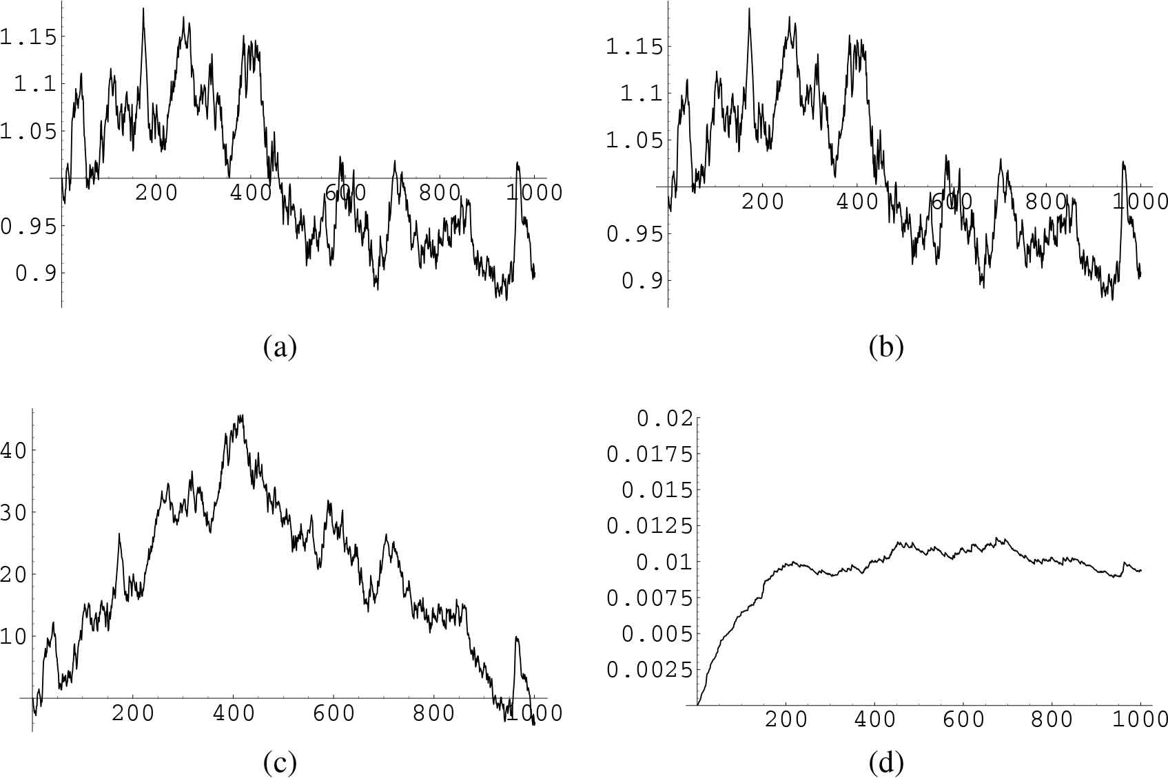
For α = β = 1, γ = 0.01, x0 = α/β (the equilibrium solution for zero noise) and a specific realization of w(t) we show: (a) the direct numerical solution x(t); (b) the solution
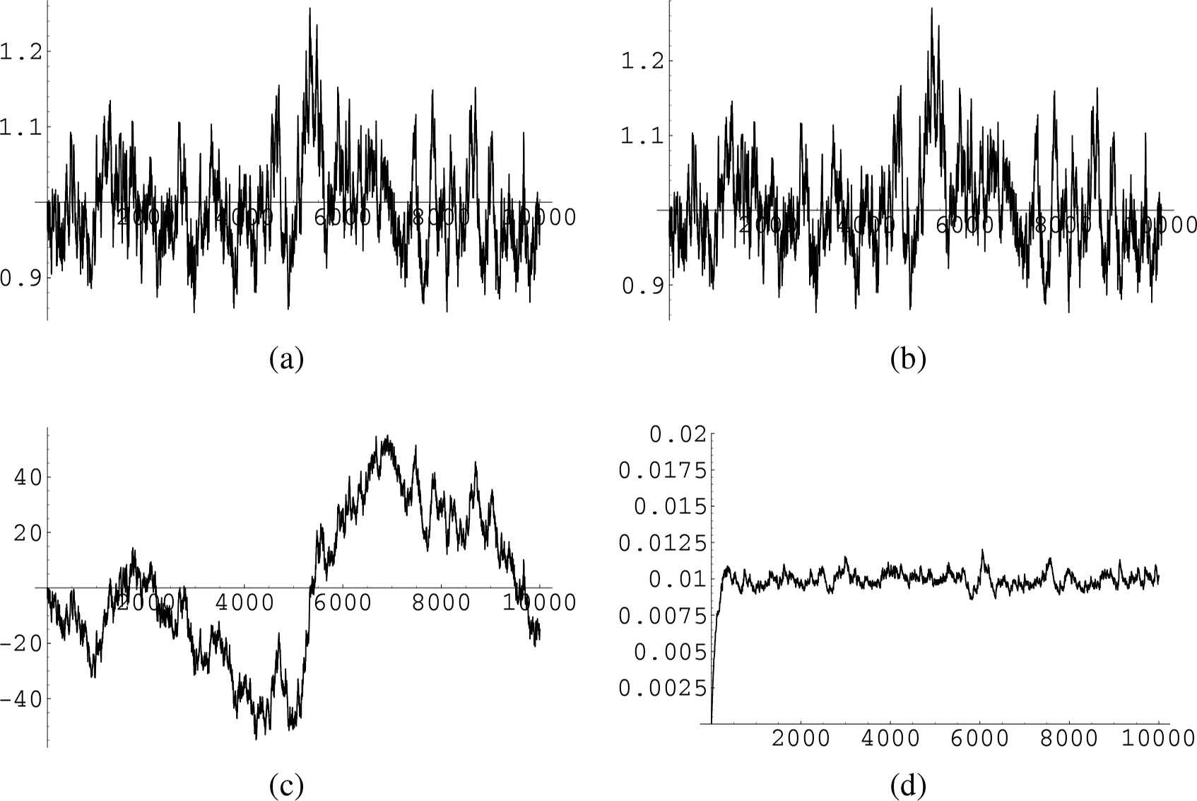
For the same parameters values as in Fig. 1 we show again: (a) x(t); (b)
7. Conclusions
We have considered the stochastic logistic equation (2.3). We have shown that in order to integrate it, i.e. to provide x(t) for given x(0) and for each realization of the Wiener process w(t) one can pass to consider the random variable y(t) defined by (5.2). This evolves according to (5.5) and is therefore given by (5.7). Going back to the original variable amounts to applying (5.3).
This allows to obtain much more precise information about solutions to (2.3); in particular one can obtain information for each realization of the driving process w(t).
We have also checked by numerical computations for different given realization of the driving process that our procedure does indeed provide a solution to the stochastic logistic equation.
Acknowledgements
Most of this work was performed over a stay at SMRI, providing as usual a relaxed atmosphere and convenient working conditions. My work is also supported by GNFM-INdAM.
Footnotes
The exact balance between the two will of course depend on the coupling constants σd, σe, so the concept of “large” will be meant in the sense x ≫ (σd/σe)2.
Any standard symmetry can also be considered, for ease of discussion, a trivial W-symmetry, with R = 0.
We also stress that, conversely, if the Ito equation (3.4) is reducible to the integrable form (3.13) by a simple random change of variables y = Φ(x, t; w) then necessarily (3.4) admits X = [Φx(x, t, w)]−1∂x := φ(x, t, w)∂x as a symmetry vector field, and when (3.13) is actually of Ito form then (3.15) is satisfied with ψ = ∂w(1/φ) [14].
More precisely, if we require that the coefficient F(t, w) of dt in (5.8) is independent of w, i.e. study the equation ∂wF = 0, we obtain the unique solution ρ(t, w) = (β/α)exp[(α − γ2/2)t + γw] + c1 exp[γw − (γ2/2)t], which yields F = 0.
We stress we are here using a very basic Euler first order integration scheme, thus have to expect rather poor precision in our numerical results. One could use more refined integration schemes – see e.g. [6] – but the point here is just to have a reference numerical solution to compare our exact solution with.
References
Cite this article
TY  - JOUR
AU  - Giuseppe Gaeta
PY  - 2021
DA  - 2021/01/06
TI  - Integration of the stochastic logistic equation via symmetry analysis
JO  - Journal of Nonlinear Mathematical Physics
SP  - 454
EP  - 467
VL  - 26
IS  - 3
SN  - 1776-0852
UR  - https://doi.org/10.1080/14029251.2019.1613052
DO  - 10.1080/14029251.2019.1613052
ID  - Gaeta2021
ER  -