
Integrable discrete autonomous quad-equations admitting, as generalized symmetries, known five-point differential-difference equations
- DOI
- 10.1080/14029251.2019.1613050How to use a DOI?
- Keywords
- Integrability; Generalized symmetries; Quad-equations
- Abstract
In this paper we construct the autonomous quad-equations which admit as symmetries the five-point differential-difference equations belonging to known lists found by Garifullin, Yamilov and Levi. The obtained equations are classified up to autonomous point transformations and some simple non-autonomous transformations. We discuss our results in the framework of the known literature. There are among them a few new examples of both sine-Gordon and Liouville type equations.
- Copyright
- © 2019 The Authors. Published by Atlantis and Taylor & Francis
- Open Access
- This is an open access article distributed under the CC BY-NC 4.0 license (http://creativecommons.org/licenses/by-nc/4.0/).
1. Introduction
In this paper we consider in discrete quad-equations. Quad-equations are four-point relations of the form:
It is known [20, 29, 31–33] that the generalized symmetries of quad-equations are given by differential-difference equations of the form:
The vast majority of quad-equations known in literature admits as generalized symmetries three-point differential-difference equations in both directions [23, 29, 32, 36, 44, 45]. When the given quad-equation admits three-point generalized symmetries it can be interpreted as a B¨acklund transformation for these differential-difference equantions [28,29]. More recently, several examples with more complicated symmetry structure have been discovered [2,10,11,14,33].
In the aforementioned papers the problem which was addressed was to find the generalized symmetries of a given quad-equation. If the generalized symmetries are given by integrable differential-difference equations, then one can construct a whole hierarchy of generalized symmetries for the given quad-equation which is integrable according to the generalized symmetries method [46]. On the other hand, also the converse problem can be considered: fixed a differential-difference equation find the quad-equation admitting it as a generalized symmetry. This point of view was taken in [31], using one well-known five-point autonomous differential-difference equation. In [15] a similar analysis was carried out for a known class of integrable non-autonomous Volterra and Toda three-point differential-difference equations [30].
In this paper we are going to generalize the results of [15, 31]: we will start from a known integrable autonomous five-point differential-differential equation and construct the quad-equation admitting it as generalized symmetry in the n direction, i.e. of the form (1.2a). To this end we will use the classification of the five-point differential-difference equations given in [18, 19]. The equations belonging to the classification in [18,19] have the following form:
This class contains fourteen equations. Equations belonging to this class are denoted by (E.x′), where x is an Arabic number. For easier understanding of the results, we split the complete list into smaller Lists 1–6. In each List the equations are related to each other by autonomous non-invertible and non-point transformations or simple non-autonomous point transformations. Moreover, for sake of simplicity, since the equations are autonomous, in displaying the equations we will use the short-hand notation ui = uk+i.
-
List 1. Equations related to the double Volterra equation:
-
Transformations ũk = u2k or ũk = u2k+1 turn equations (E.1)–(E.3) into the well-known Volterra equation and its modifications in their standard form. The other equations are related to the double Volterra equation(E.1) through some autonomous non-invertible non-point transformations. We note that equation (E.2′) was presented in [4].
-
List 2. Linearizable equations:
In both equations a ≠ 0, in (E.7) (a+1)d = bc, and T is the translation operator Tfk = fk+1.
Both equations of List 2 are related to the linear equation:
through an autonomous non-invertible non-point transformations. We note that (E.7) is linked to (1.6) with a transformation which is implicit in both directions, see [18] for more details. -
List 3. Equations related to a generalized symmetry of the Volterra equation:
These equations are related between themselves by some transformations, for more details see [19]. Moreover equations (E.3′,E.4′,E.5′) are the generalized symmetries of some known three-point autonomous differential-difference equations [46].
-
List 4. Equations of the relativistic Toda type:
Equation (E.13′) was known [12,14] to be is a relativistic Toda type equation. Since in [18] it was shown that the equations of List 4 are related through autonomous non-invertible non-point transformations, it was suggested that (E.9) and (E.10) should be of the same type. Finally, we note that equation (E.9) appeared in [1] earlier than in [18].
-
List 5. Equations related to the Itoh-Narita-Bogoyavlensky (INB) equation:
Equation (E.11) is the well-known INB equation [8,27,34]. Equations (E.12) with a = 0 and (E.13) with a = 0 are simple modifications of the INB and were presented in [33] and [9], respectively. Equation (E.13) with a = 1 has been found in [40]. Up to an obvious linear transformation, it is equation (17.6.24) with m = 2 in [40]. Equation (E.9′) is a well-known modification of INB equation (E.11), found by Bogoyalavlesky himself [8]. Finally, equation (E.11′) with a = 0 was considered in [4]. All the equations in this list can be reduced to the INB equation using autonomous non-invertible non-point transformations. Moreover, equations (E.12),(E.14) and (E.9′) are related through non-invertible transformations to the equation:
We will also study below equation (1.7), see Remark 2.2 in Section 2.
-
List 6. Other equations:
Equation (E.15) has been found in [42] and it is called the discrete Sawada-Kotera equation [2, 42]. Equation (E.14′) is a simple modification of the discrete Sawada-Kotera equation (E.15). Equation (E.16) has been found in [1] and is related to (E.15). On the other hand equation (E.17) has been found as a result of the classification in [18] and seems to be a new equation. It was shown in [16] that equation (E.17) is a discrete analogue of the Kaup-Kupershmidt equation. Then we will refer to equation (E.17) as the discrete Kaup-Kupershmidt equation. No transformation into known equations of equation (E.17) is known.
As a result we will obtain several examples of autonomous nontrivial quad-equations. By non-trivial equations we mean non-degenerate, irreducible and nonlinear equations. Moreover we consider as trivial also the equations
We underline that, by construction, all the equations we are going to produce will possess a generalized symmetry in the n direction (1.2a) which is not sufficient for integrability. To prove that the equation, we are going to produce, are LT or sGT we will either identify them with known equations, or present their first integrals in the sense of (1.9) or a generalized symmetry in the m direction (1.2b).
The plan of the paper is then the following: In Section 2 we discuss the theoretical background which allows us to make the relevant computations. In Section 3 we enumerate all the quad-equations of the form (1.1) which corresponds to the equations of the Class I and II and describe their properties. Finally in Section 4 we give a summary of the work and some outlook for future works in the field.
2. The method
The most general autonomous multi-affine quad-equation has the following form:
From (1.2a) and (1.3) we have that the most general symmetry in the n direction of the form (1.2a) belonging to Class I and II can be written as:
We have then the following general result, analogous to Theorem 2 in [15]:
Theorem 2.1.
If the autonomous quad-equation (2.1) admits a generalized symmetry of the form (2.2) then it has the following form:
Proof.
By multi-linearity we can always solve (2.1) with respect to un+1,m+1 and write:
From Theorem 2 in [31] we have that a quad-equation admits a generalized symmetry of the form (1.2a) with k1 = − k′1 = 2 if the following conditions are satisfied:
In (2.5) we suppressed the indices n, m in φ since we are dealing with autonomous differential-difference equations. Now from (2.2) we have:
From equation (2.6) we have differentiating (2.5a) w.r.t. un+2,m:
Therefore we get the two conditions:
Working out explicitly the conditions in (2.9) and using (2.1) we obtain:
Relabeling the parameters as
Remark 2.1.
We note that the condition (2.9) is the same as formula (29) in [15] even though the class of considered differential-difference equation is different.
Remark 2.2.
It can be proved in a similar way that Theorem 2.1 is valid for generalized symmetries of the form (1.2a) satisfying the conditions k′1 = k1 and
Theorem 2.1 tells us that the most general form of a quad-equation admitting a five-point generalized symmetry in the n direction of the form (2.2) is given by (2.3). At this point we can pick up any of the members of Class I and II and follow the scheme of [18, App. B], i.e. we fix a specific form of a, b and c in (2.2). We beging by imposing the exponential integrability conditions (2.5a) and (2.5b) and finally we impose the symmetry condition:
Taking the numerator of (2.13) we obtain a polynomial in the independent variable (2.14). This polynomial must be identically zero, so we can equate to zero all its coefficients.
This lead us to a system of algebraic equation in the coefficients of the multi-affine function (2.3). Doing so we reduce the problem of finding a quad-equation admitting a given five-point symmetry of the form (2.2) to the problem of solving system of algebraic equations. Such system can be solved using a Computer Algebra System like Maple, Mathematica or Reduce. Amongst the possible solutions of the system we choose the non-degenerate ones. The non-degeneracy condition is the following one:
Note that this non-degeneracy condition includes the requirement that a quad-equation must be given by an irreducible multi-affine polynomial, see the introduction.
Remark 2.3.
Several equations in Class I and II, e.g. (E.5) or (E.5′), depend on some parameters. Depending on the value of the parameters there can be, in principle, different quad-equations admitting the given differential-difference equation as five-point generalized symmetries. When possible, in order to avoid ambiguities and simplify the problem, we use some simple autonomous transformations to fix the values of some parameters. The remaining free parameters are then treated as unknown coefficients in the system of algebraic equations. We will describe these subcases when needed in the next section.
The number of the resulting equations is then reduced using some point transformations. These point transformations are essentially of two different kind: non-autonomous transformations of the dependent variable un,m:
Now, in the next section we describe the results of this search.
3. Results
In this section we describe the results of the procedure outlined in Section 2. Specifically, as described in 2.3 we will explicit the particular cases in which the parametric equations can be divided.
3.1. List 1
Equation (E.1): To equation (E.1) correspond only degenerate quad-equations in the sense of condition (2.15).
Equation (E.2): To equation (E.2) correspond two nontrivial quad-equations:
Up to transformation (T.1) we can reduce these two equations to only one, say the one with a = −i. Equation (3.1, a = −i) is a special case of equation (7) with a2 = −i of List 4 in [14]. This means that this is a LT equation, its first integrals being:
See [14] for more details.
Equation (E.3): To equation (E.3) correspond only degenerate quad-equations in the sense of condition (2.15).
Equation (E.4): To equation (E.4) correspond only degenerate quad-equations in the sense of condition (2.15) or the linear discrete wave equation:
Equation (E.5): Equation (E.5) depends on the parameters a and b. If a ≠ 0 it is possible to scale it to one through a scaling transformation. This amounts to consider the cases a = 1 and a = 0.
To equation (E.5, a = 1) correspond only degenerate quad-equations in the sense of condition (2.15) or the linear discrete wave equation (3.3). The same holds true for equation (E.5, a = 0). So to all the instances of equation (E.5) correspond only trivial or linear equations.
Equation (E.6): To equation (E.6) correspond two quad-equation. One is the trivial exponential wave equation (1.8a), while the other one is the LT equation:
Equation (3.4) is equation (9) with c4 = 1 of List 4 in [14]. Its first integrals are [14]:
Equation (E.1′): To equation (E.1′) correspond only degenerate quad-equations in the sense of condition (2.15) and the trivial linearizable equation (1.8a).
Equation (E.2′): Equation (E.2′) is very rich, since it give raise to many different equations. We have two trivial linearizable equations of the form (1.8a), but also twelve nontrivial equations. We have four equations of the form:
Then four equations of the form:
Finally we have four equations of the form:
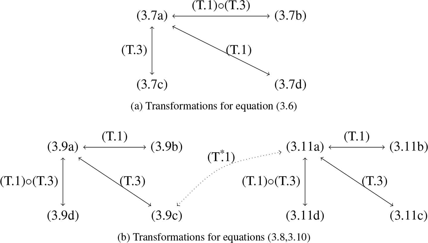
Up to the transformations (T.1,T.3) and (T*.1) we can reduce equations (3.6,3.8,3.10) to only two equations, say (3.6) with the parameters (3.7d) and (3.8) with the parameters (3.9d):
For a complete description of the transformations leading to (3.12) see Figure 1.
Equation (3.12a) is a LT equation. It can identified with equation (7) with a2 = 1 of List 4 of [14]. In particular its first integrals are given by:
Equation (3.12b) is a LT equation too. Its first integrals are given by:
Note that the W2 first integral of (3.12b) is very similar to the W2 first integral of (3.12a). Moreover, the W1 first integral of (3.12b) is a generalization of the W1 first integral of (3.12a) with more points. It is possible to show that equation (3.12b) do not belong to known families of Darboux integrable equations [5, 14, 24, 37, 38], because of the specific form of W1. Therefore we believe that equation (3.12b) is a new Darboux integrable equation.
3.2. List 2
Equation (E.7): Equation (E.7) depends on four parameters a, b, c and d linked among themselves by the condition (a+1)d = bc. Therefore we have that using a linear transformation un,m → αun,m + β we need to consider only three different cases: 1) a ≠ 0, a ≠ −1, b = 0, d = 0, 2) a = −1, b = 1, c = 0, 3) a = −1, b = 0 (recall that a ≠ 0 in all cases).
Case a ≠ 0, a ≠ −1, b = 0, d = 0: For these values of the parameters we obtain either linear equations or exponential wave equations (1.8b) if also a ≠ 1 and c ≠ 0. For a = 1 and c = 0 we obtain the equation:
In equation (3.15) we have the condition c3d3d4 ≠ 0. Using a linear transformation of the form un,m = Aûn,m + B we can reduce equation (3.15) to two different cases.
-
Case 1: If
This equation is equation (1) of List 3 of [14], hence it is a LT equation with the following first integrals:
-
Case 2: If
and equation (3.15) reduces to:This equation is equation (3) of List 3 of [14] with
-
Case a = −1,b = 1,c = 0: For this value of the parameters only degenerate or linear equations arise. In particular we have discrete wave-like equation.
-
Case a = −1, b = 0: For this value of the parameters we have several linear wave-like equations, but also one nontrivial equation:
where we have the following relationship between the parameters:The case b4 = −d3 (3.21) is equivalent to (1.8) up to a linear transformation. The case b4 ≠ −d3, c = d = 0, and (3.21) is equavalent to (4) of List 4 of [14] up to a linear transformation and it is a LT equation.
Equation (E.8): To equation (E.8) correspond only degenerate quad-equations in the sense of condition (2.15) and the trivial linearizable equation (1.8b).
3.3. List 3
Equation (E.3′): To equation (E.3′) correspond only degenerate quad-equations in the sense of condition (2.15) and the trivial linearizable equation (1.8a).
Equation (E.4′): Equation (E.4′) depends on the parameters a and c. If a ≠ 0 then it can always be rescaled to 1, hence we can consider two independent cases: a = 1 and a = 0.
However, to equation (E.4′) with a = 0 correspond only degenerate quad-equations in the sense of condition (2.15) and the trivial linearizable equation (1.8a).
On the other hand, the case when a = 1 admits nontrivial solutions. Indeed, to equation (E.4′) with a = 1 correspond eight nontrivial equations. Four of them are valid for every value of c:
Using the transformation un,m → −un,m we can reduce the (3.23,−σ1 = σ2 = 1) case to the (3.23,σ1 = −σ2 = 1) case and the (3.23,σ1 = σ2 = −1) case to the (3.23,σ1 = σ2 = 1) case respectively. This means that we have only the two following independent equations
Other four equations are found if c = −4:
Using the transformation un,m → −un,m we can reduce the (3.25,−σ1 = σ2 = 1) case to the (3.25,σ1 = −σ2 = 1) case and the (3.25,σ1 = σ2 = −1) case to the (3.25,σ1 = σ2 = 1) case respectively. This means that we have only the two following independent equations
Equation (3.24a) is a well-known sGT equation. It corresponds to equation T1* in [32]. See references therein for a discussion of the appearance of this equation in literature. On the other hand equation (3.24b) is transformed into equation (3) of List 4 in [14] with the linear transformation un,m = 2ûn,m + 1. This means that this equation is a known LT equation with the following first integrals:
For further details see [37].
Equation (3.26a) is a new example of LT equation and has first integrals:
The integral W2 is a sixth order (seven-point) first integral. It can be proved that there is no first integral of lower order in this direction. Examples of equations with first integrals of such a high order, except for a special series of Darboux integrable equations presented in [13], are, at the best of our knowledge, new in the literature.
Now we are going to use a transformation theory presented in [37, 47]. We can rewrite (3.26a) in a special form and introduce a new function vn,m as follows:
So we have
This is a non-point transformation which is invertible on the solutions of (3.26a). Formula (3.30) allows to rewrite (3.26a) as
Both first integrals (3.32) are of lowest possible order in their directions. Example (3.31) is still exeptional, even though the order of W2 has been lowered to five.
Equation (3.26b) is a sGT equation, as we can prove that it possesses the following second order autonomous generalized symmetries in both directions:
It can be proved by direct computation using the method of [20, 31, 32] that equation (3.26b) does not admit any autonomous generalized symmetries of lower order. Equation (3.26b) seems to be a new interesting example and deserves a separate study, see [17].
Here we limit ourselves to observe that equation (3.26b) is an integrable equation according to the algebraic entropy test [7,41,43]. Indeed, computing the degree of the iterates of equation (3.26b) by using the library <monospace>ae2d.py</monospace> [21,22], we obtain the following sequence:
The sequence (3.35) is fitted by the following generating function:
Since the generating function (3.36) has only one pole in z0 = 1 and it lies on the unit circle, equation (3.26b) is integrable according to the algebraic entropy criterion. Moreover, due to the presence of (z − 1)3 in the denominator of the generating function (3.36) we have that growth of equation (3.26b) is quadratic. According to the classification of discrete equations using algebraic entropy [26] we have that equation (3.26b) is supposed to be genuinely integrable and not linearizable.
Equation (E.5′): To equation (E.5′) with a ≠ 0 corresponds one quad-equation:
When a = 0, to equation (E.5′) corresponds two quad-equations. One of them is just (3.37) with a = 0, and the second one is:
For any a equation (3.37) is transformed into (T4) of [32] by the following non-autonomous linear point transformation:
We recall that equation (T4) is a sGT equation, with two nontrivial three-point generalized symmetries [32].
In the same way equation (3.38) is another sGT equation which is transformed by linear transformation of un,m into the special form:
This equation is a new sGT quad-equation which possesses five-point autonomous generalized symmetries:
We note that equation (3.38) possesses also the following non-autonomous three-point generalized symmetry in the n-direction:
On the other side it is possible to prove by direct computation using the method of [20, 31, 32] that no three-point generalized symmetry exists in the m-direction. Hence the generalized symmetry (3.41b) is the lowest order generalized symmetry of equation (3.38) in the m-direction.
We remark that equation (3.38) through the following nontrival non-invertible transformation:
Finally, we underline that equation (3.41b) is a particular case of known example of integrable five-point differential-difference equation presented in [3]. According to this remark we have that equation (3.33b) is a nontrivial modification of a known example.
Equation (E.6′): To equation (E.5) correspond only degenerate quad-equations in the sense of condition (2.15) and the trivial linearizable equation (1.8a).
Equation (E.7′): Equation (E.7′) depends on the parameter a. If a ≠ 0 then it can always be rescaled to 1, hence we can consider two independent cases: a = 1 and a = 0. However, in both cases to equation (E.7′) corresponds only degenerate quad-equations in the sense of condition (2.15).
Equation (E.8′): To equation (E.5) correspond only degenerate quad-equations in the sense of condition (2.15) and the trivial linearizable equation (1.8a).
3.4. List 4
Equation (E.9) To equation (E.9) correspond only degenerate quad-equations in the sense of condition (2.15).
Equation (E.10) To equation (E.10) correspond only degenerate quad-equations in the sense of condition (2.15) and equations of the form of the linear discrete wave equations (3.3).
Equation (E.13′): To equation (E.13′) correspond two nontrivial equations:
Equation (3.46b) can be reduced to equation (3.46a) using the transformation (T*.1). Using the scaling
No autonomous three-point symmetry exists for equation (3.46a).
3.5. List 5
Equation (E.11) To equation (E.11) correspond only degenerate quad-equations in the sense of condition (2.15).
Equation (E.12) Equation (E.12) depends on two parameters a and b. If a ≠ 0 it can always be scaled to a = 1, so for this equations we get two different cases: when a = 1 and when a = 0.
Case a = 1: For this value of the parameter only degenerate or linear equations arise. In particular we have a discrete wave equation (3.3).
Case a = 0: For this value of the parameter only degenerate or linear equations arise. In particular we have a discrete wave equation (3.3).
Equation (E.13) Equation (E.13) depends only on the parameter a. If a ≠ 0 it can be scaled to a = 1 always. Therefore we have to consider the cases a = 1 and a = 0.
Case a = 1: For this value of the parameter there are two nontrivial equations:
Up to transformation (T*.1) we have that equation (3.50b) reduces to equation (3.50a). Therefore we have only one independent equation. Equation (3.50a) is a sGT equation and appeared as formula (58) in [33].
Case a = 0: For this value of the parameter there are six nontrivial equations:
Up to transformations (T.1), (T.2) and(T*.1) we have that all the equations in (3.51) can be reduced to (3.51a). The precise relationship between these equations is illustrated in Figure 2. Equation (3.51a) is a known LT equation and it can be identified with (6) with a2 = 1 of List 4 of [14]. Its first integrals are:
The relationship between the equations (3.51). By (T.1)◦(T.2) we mean the composition of the two transformations.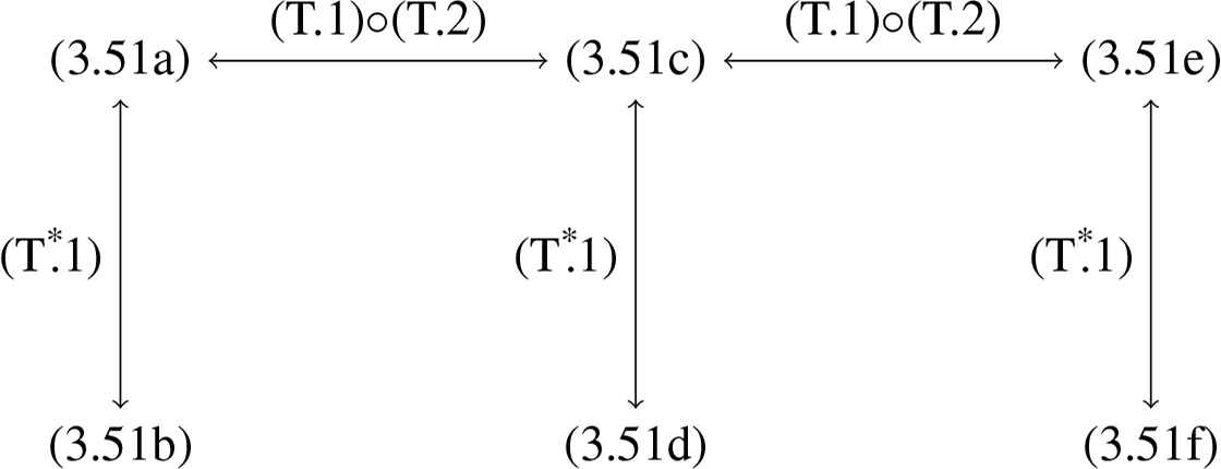
Equation (E.14): To equation (E.14) correspond only degenerate quad-equations in the sense of condition (2.15).
Equation (1.7): To equation (1.7) correspond three nontrivial quad-equationsa:
Equation (3.53a) is a LT equation. Using the transformation
Equation (3.53b) under the non-autonomous transformation
Equation (E.9′): To equation (E.9′) correspond only degenerate quad-equations in the sense of condition (2.15) and the trivial linearizable equation (1.8a).
Equation (E.10′): Equation (E.10′) depends on the parameter a. If a ≠ 0 then it can always be rescaled to 1, hence we can consider two independent cases: a = 1 and a = 0. However in both cases to equation (E.9′) correspond only degenerate quad-equations in the sense of condition (2.15) or linear equations of the form of the discrete wave equation (3.3).
Equation (E.11′): Equation (E.11′) depends on the parameter a. If a ≠ 0 then it can always be rescaled to 1, hence we can consider two independent cases: a = 1 and a = 0.
To equation (E.11′) when a = 1 correspond four nontrivial equations:
Up to transformations (T*.1,T.1) we have that all the equations in (3.58) can be reduced to (3.58a), see Figure 3. Equation (3.58a) is a known equation. It was introduced in [25], while in [10] it was proved that it is a sGT equationb.
The relationship between the equations (3.58). By (T*.1)◦(T.1) we mean the composition of the two transformations.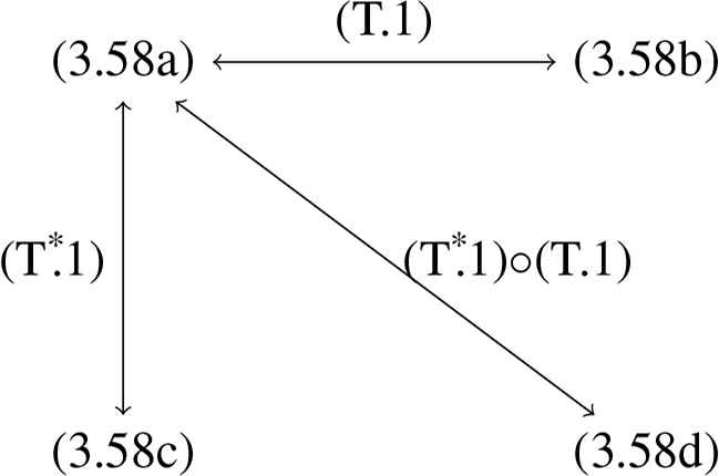
To equation (E.11′) when a = 0 correspond twelve nontrivial equations. Six of them are those of presented in formula (3.51), but we also have the following six other equations:
Using the transformations (T*.1,T.1,T.2) we have that the only independent equation is (3.51a). See Figure 4 for the details about the needed transformations. As discussed above equation (3.51a) is a LT equation with known first integrals (3.52).
The relationship between the equations (3.59) and (3.51a). By (T.1)◦(T.2) we mean the composition of the two transformations.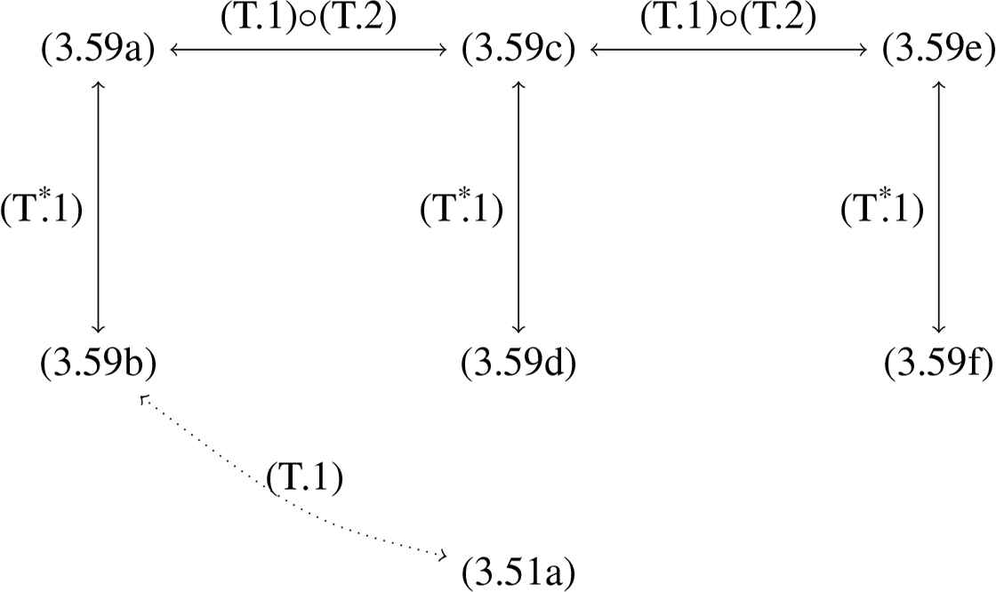
Equation (E.12′): To equation (E.12′) correspond only degenerate quad-equations in the sense of condition (2.15) or the trivial linearizable equation (1.8a).
3.6. List 6
Equation (E.15): To equation (E.15) correspond only degenerate quad-equations in the sense of condition (2.15).
Equation (E.16): To equation (E.16) correspond only degenerate quad-equations in the sense of condition (2.15).
Equation (E.17): Equation (E.17) is not rational, so we are not going to consider it as we are dealing with multi-affine quad-equations (2.3). It can be remarked that equation (E.17) has as a rational form, but it is quadratic in uk±2, so it is outside the main class of differential-difference equations.
Equation (E.14′): To equation (E.14′) correspond only degenerate quad-equations in the sense of condition (2.15) or equations of the form of the linear discrete wave equation (3.3).
4. Summary and outlook
In this paper we have constructed all the possible autonomous quad-equations (1.1) admitting, as generalized symmetries, some known five-point differential-difference equations belonging to a class recently classified in [18,19].
In section 2 we gave a general result on all the quad-equations admitting a generalized symmetry of the form (2.2), resulting in the simplified form (2.3). Then in section 3 we considered all the explicit examples of five-point differential-difference equations and found all the corresponding quad-equations. We discussed the properties of these equations, highlighting which are LT and which are sGT equations. We present a summary of these properties in Table 1. Referring to the table, we have that the majority of the differential-difference equations of the form (1.3) as classified in [18, 19] give raise to degenerate or trivial quad-equations. However eight of them give also rise to LT equations. Most of these LT equations were known, but we also obtained two new LT equations, namely equations (3.12b) and (3.26a). Moreover, as expected, sGT equations are even rarer, appearing only in in four examples. Among these sGT equations there are two new examples, namely equations (3.26b) and (3.40). In this paper we limited ourselves to present the result of the algebraic entropy test for equation (3.26b), which suggests integrability. More details and generalizations, including L − A pairs, on equation (3.26b) can be found in [17].
| Class I | Class 2 | ||
|---|---|---|---|
| Equations | Properties | Equations | Properties |
| (E.1) | Trivial | (E.1′) | Trivial |
| (E.2) | LT | (E.2′) | LT* |
| (E.3) | Trivial | (E.3′) | Trivial |
| (E.4) | Trivial | (E.4′,a = 1) | sGT*, LT* |
| (E.5, a = 1) | Trivial | (E.4′,a = 0) | Trivial |
| (E.5, a = 0) | Trivial | (E.5′) | sGT* |
| (E.6) | LT | (E.6′) | Trivial |
| (E.7, a ≠ 0,±1,b = d = 0,c ≠ 0) | Trivial | (E.7′, a = 1) | Trivial |
| (E.7, a = 1,b = c = d = 0) | LT | (E.7′, a = 0) | Trivial |
| (E.7, a = −1,b = 1,c = 0) | Trivial | (E.8′) | Trivial |
| (E.7, a = −1,b = 0) | LT | (E.9′) | Trivial |
| (E.8) | Trivial | (E.10′, a = 1) | Trivial |
| (E.9) | Trival | (E.10′, a = 0) | Trivial |
| (E.10) | Trivial | (E.11′, a = 1) | sGT |
| (E.11) | Trivial | (E.11′, a = 0) | LT |
| (E.12, a = 1) | Trivial | (E.12′) | Trivial |
| (E.12, a = 0) | Trivial | (E.13′) | sGT |
| (E.13, a = 1) | sGT | (E.14′) | Trivial |
| (E.13, a = 0) | LT | ||
| (E.14) | Trivial | ||
| (E.15) | Trivial | ||
| (E.16) | Trivial | ||
| (E.17) | Not rational | ||
| (1.7) | LT | ||
Summary of the properties of the corresponding discrete quad-equations. With * we underline the presence of new quad-equations.
It should be remarked that in [35,39,40] some more general completely discrete equations consistent with the INB-like five-point differential-differential equations were studied. In the mentioned papers a natural discretization based on the B¨acklund transformation was presented and it had the form:
This is an equation on two adjacent quads. Quad equations (1.1) like we consider in this paper are also determined by B¨acklund transformations, but of a quite different form. Quad equations (1.1) might be special reductions of equations of the form (4.1) as well of the corresponding B¨acklund transformations.
As we remarked at the beginning of this section, in this paper we only dealt with autonomous differential-difference equations and autonomous quad-equations. We are now working on weakening this condition for the fully discrete equations to present a classification of non-autonomous quad-equations admitting the differential-difference equations found in [18, 19] as five-point generalized symmetries. This classification can be performed with the method presented in [15] and applied to some known autonomous and non-autonomous three-point differential-difference equations of Volterra and Toda type.
Acknowledgment
GG is supported by the Australian Research Council through Nalini Joshi’s Australian Laureate Fellowship grant FL120100094.
We thank the anonymous referee for the interesting comments on the discretization of the INB-like equations.
Footnotes
By direct computations several sub-cases of equations (3.53) are found. We omit them since they are not independent cases.
Therein it is given by equation (1.9).
Bibliography
Cite this article
TY  - JOUR
AU  - Rustem N. Garifullin
AU  - Giorgio Gubbiotti
AU  - Ravil I. Yamilov
PY  - 2021
DA  - 2021/01/06
TI  - Integrable discrete autonomous quad-equations admitting, as generalized symmetries, known five-point differential-difference equations
JO  - Journal of Nonlinear Mathematical Physics
SP  - 333
EP  - 357
VL  - 26
IS  - 3
SN  - 1776-0852
UR  - https://doi.org/10.1080/14029251.2019.1613050
DO  - 10.1080/14029251.2019.1613050
ID  - Garifullin2021
ER  -