
Evaluation of the Relationships between Saliency Maps and Keypoints
- DOI
- 10.2991/jrnal.k.200512.004How to use a DOI?
- Keywords
- Saliency map; binary robust invariant scalable keypoint; keypoint stability
- Abstract
The saliency map is proposed by Itti et al., to represent the conspicuity or saliency in the visual field and to guide the selection of attended locations based on the spatial distribution of saliency, which works as the trigger of bottom-up attention. If a certain location in the visual field is sufficiently different from its surrounding, we naturally pay attention to the characteristic of visual scene. In the research of computer vision, image feature extraction methods such as Scale-Invariant Feature Transform (SIFT), Speed-Up Robust Features (SURF), Binary Robust Invariant Scalable Keypoint (BRISK) etc., have been proposed to extract keypoints robust to size change or rotation of target objects. These feature extraction methods are inevitable techniques for image mosaicking and Visual SLAM (Simultaneous Localization and Mapping), on the other hand, have big influence to photographing condition change of luminance, defocusing and so on. However, the relation between human attention model, Saliency map, and feature extraction methods in computer vision is not well discussed. In this paper, we propose a new saliency map and discuss the stability of keypoints extraction and their locations using BRISK by comparing other saliency maps.
- Copyright
- © 2020 The Authors. Published by Atlantis Press SARL.
- Open Access
- This is an open access article distributed under the CC BY-NC 4.0 license (http://creativecommons.org/licenses/by-nc/4.0/).
1. INTRODUCTION
In recent years, many attempts have been done such as the selection of desired information in input information [1,2]. If attention models can be constructed to select information, the intelligence and awareness of humans can be implemented in computers.
According to Itti et al., saliency is defined as the property of images, which triggers bottom-up attentions. Saliency occurs by the local conspicuity over the entire visual scene [3]. In this model (Figure 1), input image is decomposed into luminance, color, and orientation components, then, each component is processed individually with Gaussian filter.
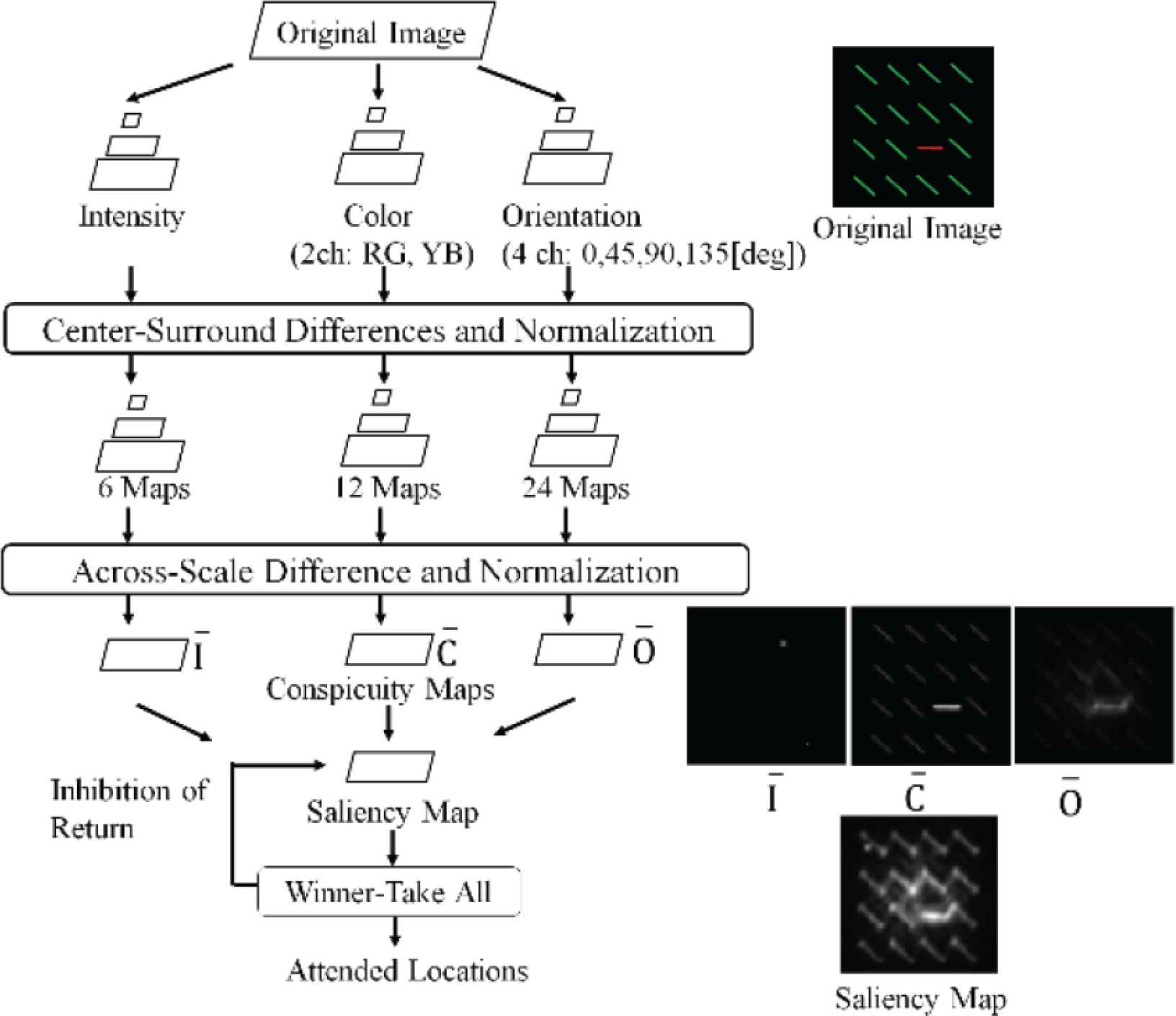
Itti’s saliency map.
Considering that the saliency map is applied to environment recognition by mobile robots, various changes in photographing condition are expected to affect the input image. The change affects spatial frequency components of the image. If the spatial frequency changes, the response of Gaussian filter also changes, then, the effect reflects saliency map. Considering that the saliency map is used to select the keypoints of the image, changes in the saliency map affect the results of feature selection, then, input data of detectors vary. Thus, recognition results are influenced according to the change in photographing conditions.
For keypoint extraction, small influence is desirable in spite of the variety of object size, angle and luminance. In case of the keypoint application for object detection, repetitively extracted keypoints are ideal to select.
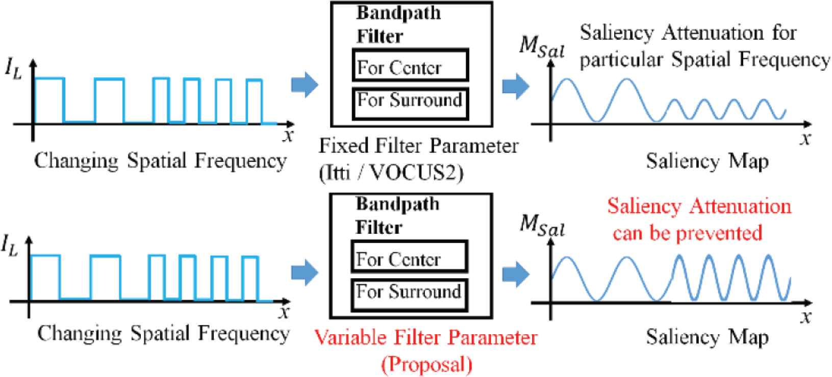
In our research, we propose a method for generating saliency maps, which can absorb the effect of spatial frequency changes. If the parameters of the filters can be determined automatically, the effect of the spatial frequency change can be diminished in saliency maps (Figure 2 Bottom). We evaluated the relationship between saliency and keypoints.
Adjustment of smoothing filters under saliency map generation against changing spatial frequency.
2. RELATED WORK
2.1. Saliency Map
Itti et al. [3] simulated human eye movement, and expressed the result as saliency maps (Figure 1). In the process of saliency map creation input image is reduced by 1/2n and nine resolutions of the images are obtained. The Center and the Surround can be obtained through the smoothing operation by a common Gaussian filter. This signal process is similar to the different responses from fovea and its neighbor in retina for the common stimuli. All the reduced images are enlarged to the same size, and the across scale difference image of the two components is normalized and added to obtain a map for each component (i.e. Luminance, Color, Orientation). Saliency map is obtained through the addition of all the maps of the three components.
According to Frintrop et al. [4], saliency map changes if the parameter of the Gaussian filters are changed. The ratio of filter parameter σc/σs is crucial for the determination of saliency. Arbitral selection of σc/σs enabled high granularity in saliency map. However, in Itti et al. [3] and Frintrop et al. [4], the parameters cannot be adjusted depending on the variety of spatial frequency. As the result, saliency map can be affected in the event of spatial frequency change (Figure 2 Top).
2.2. Keypoint Extraction
Keypoint extraction is often applied for object recognition tasks [5], image stitching tasks [6], etc. by robot vision. A keypoint has a co-ordinate, a descriptor which explains brightness gradient in the neighborhood. In the object recognition task, the database image and the newly observed image are searched. Recently, scale-invariant keypoint extraction methods have been proposed, such as SIFT [7], and Binary Robust Invariant Scalable Keypoints (BRISK) [8] (Figure 3). As the result, the stability of object detection has been improved. However, if photographing conditions (brightness of the environment, size of the observed object, focusing conditions, camera internal parameters, etc.) change, the number of extracted keypoints changes significantly. Stably extracted keypoints are desirable for the use of object detection tasks by robot vision.

BRISK Keypoint Extraction Process.
3. PROPOSAL OF SALIENCY MAP
3.1. Outline
In this research, we developed the theory of Frintrop et al. [4] to mitigate the effect of spatial frequency variation. The strategy is automatic adjustments of σc and σs. In the saliency map generation process (Figure 4), the input image is decomposed into luminance, color, and orientation components in advance. For each component, the Center and the Surround are generated by the combination of integral image and box filters. The parameter of the filters are automatically adjusted so that the pixel values of the across scale difference are maximized. The across scale differences of all three components are merged to form saliency map.

Overview of proposed saliency map method.
3.2. Decomposition of Input
We utilize CIE-Lab color system to simplify the difference of complimentary color channel. IL, Ia and Ib indicates luminance, color (Red-Green), color (Blue-Yellow) component, each other. For the obtainment of orientation component, Haar-Like Filters (Figure 5 [9,10]) are convoluted on IL. The operations are expressed as Equation (1).
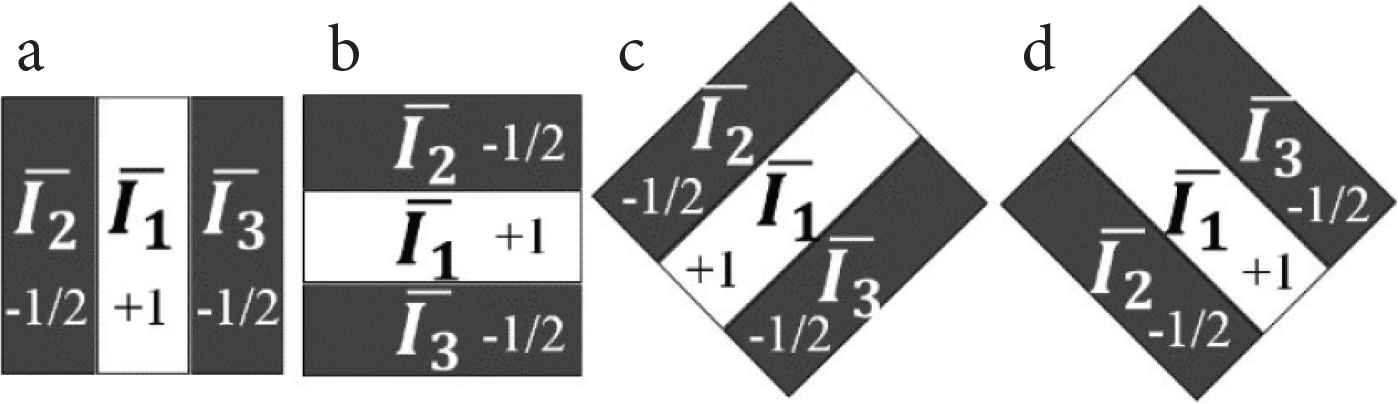
Haar-like Filters. (a) 0°, (b) 90°, (c) 90°, (d) 135°.
3.3. The Center and Surround
We align two box filters FBs, FBc centered with point pρ as shown in Figure 6. The filters are used for convolution to generate the Center and Surround. The filter widths WBs, WBc can be variable up to Wpmax and fulfills WBs > WBc. This arrangement is same as Mochizuki et al. [11].

Alignments of box filters.
3.4. Filter Adjustment
To obtain across scale difference of luminance, color components, we maximize the pixel value of the difference Ics(pp) as in Mochizuki et al. [11] by changing WBs(pp), WBc(pp) according to Equation (2) and Figure 6.
Here, WBs (pp), WBc (pp) satisfies
On the other hand, for orientation component, to obtain across scale differences the sizes of the Haar-like Filters are set to
3.5. Saliency Map Generation
Map MC (for Color), and MO (for Orientation) are obtained by Equations (4) and (5). Saliency map MSal is formed through the merge of MI, MC, MO with Eq. (6). The functions fmix, gmix, hmix for merging maps can be selected arbitrarily.
4. EVALUATION OF THE RELATIONSHIP BETWEEN SALIENCY AND KEYPOINT EXTRACTION
4.1. Outline of the Experiment
In this experiment, we assume that the selected image keypoints are used for object detection. Thus, we evaluate the relationship between saliency MSal and feature stability FStb. Suppose the number of small regions is Nq, FStb and MSal are expressed in line vector of Nq dimensions. However, we treat MSal and FStb as two dimensions (Figure 7). Then, we calculate the relationship ϕi by obtaining inner product FStb · MSal. The saliency maps were generated by conventional methods (i.e. Itti method, VOCUS2) and our proposal to compare ϕi. The source codes for the experiment are Simpsal [12] by Caltech for Itti method, and [13] for VOCUS2. We chose BRISK [8] as keypoint extraction method because descriptor is expressed in binary system. Such system is reported to require shorter time for matching than SIFT [7]. Furthermore, the descriptor has properties of rotation and scale invariance.
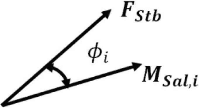
Relationship between keypoint stability FStb and saliency MSal, i.
4.2. Evaluation Function
We consider two conditions of keypoints which have high stability under photographing condition variety. First, the keypoints must extracted at the same location. We define the property as repeatability. Second, the descriptors must remain the same, that is, the similarity.
To evaluate keypoint stability, keypoint displacement have to be considered because of image flicker, resize of observed object size. For example, the combination of the same keypoints is considered as (I) or (II) in Figure 8 in different photographing condition. We define a small region of Wq × Hq [Pixels] to search identical keypoints.
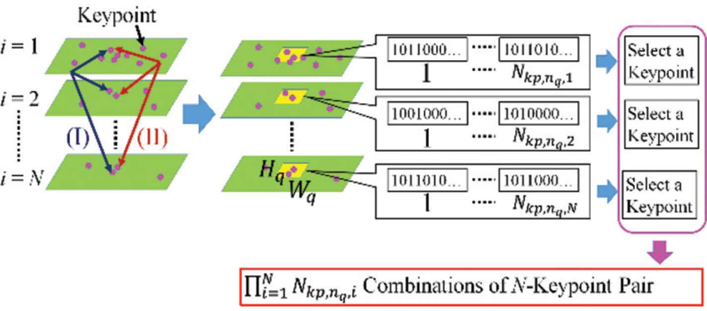
Ambiguity in keypoint identification under changing photographing condition.
Suppose Nkp,nq, i keypoints are extracted at nq-th small region under i-th photographing condition, the variance σkp, nq of keypoint number is obtained by Equation (7). The average
To obtain similarity, we select two keypoints from the same small region (as seen in Figure 8) and different photographing conditions, then calculate Hamming distance between the two descriptors. To obtain average Hamming distance of all combinations of the keypoint pairs, we use Equation (10). The similarity sDsc,nq is calculated with normalization by Equation (11) so that the range satisfies [0,1], and rDerr, nq is smaller as the distance is larger.
Keypoint stability of FStb,nq is calculated by the weighting of rDerr,nq and sDsc,nq as shown in Equation (12).
For the saliency MSal,i,nq, The maximum response of MSal is searched within each small region. Maximum saliency and feature stability are expressed as Nq dimensions of line vectors (denoted as MSal,i, FStb, respectively). ϕi is calculated as the angle between the two vectors [Equation (13)]. To be noted that rftr, sDsc are calculated only for the regions where keypoints are extracted more than twice during N variations of photographing conditions.
The average
4.3. Method
Figure 9 shows the experimental images (Lenna, Flower, Tree, Things). These images were selected in the database of Caltech [14] and Standard Image Data BAse (SIDBA) [15]. The spatial frequency spectrums of the images are shown in Figure 10. Lenna is well known for test image to be used image analysis. Flower has wider spectrum than Lenna with higher frequency component. As well as the comparison of Things and Tree, Things has higher frequency component than Tree.


Spectrum of spatial frequency which FFT algorithm returns as spatial frequency components. u = v = 256 for DC component. The brightness means the intensity of the component.
The photographing condition to adjust to vary extracted keypoint number is IMax,i/IMax,1 for luminance, WObj,i/WObj,1 for object size, each other, whose range is from 0.5 to 1.0 with the step 0.1 of increase.
For changing WObj,i, we selected images of no white background, (i.e. Tree and Flower). We selected TFAST = 20 (TFAST: Threshold of FAST Score [8]) and IMax,1 = 255 during the adjustment of IMax,i and WObj,i. As the setting of the proposal, for Setting 1, Wpmax = WIM/4 and for Setting 2, Wpmax = WIM / 2. WIM indicates the image width. The resolution of the image is WIM × HIM = 512 × 512 [Pixel].
4.4. Results and Discussion
Tables 1 and 2 shows the relationship of MSal, rftr and MSal, sDsc under variable IMax, i, and WObj,i, each other. Flower has higher frequency component than Lenna, and Things has higher frequency component than Tree.
| (a) w = 1 (FStb = rftr) | |||||
| Image | VOCUS2 | Itti | Proposal | ||
| 1/10 | 5/10 | Set 1 | Set 2 | ||
| Lenna | 18.13 | 20.63 | 31.61 | 19.94 | 18.04 |
| Flower | 29.00 | 29.64 | 41.39 | 19.72 | 18.98 |
| Tree | 21.85 | 24.34 | 33.97 | 20.76 | 20.10 |
| Things | 31.24 | 29.77 | 28.36 | 19.60 | 18.37 |
| (b) w = 0 (FStb = sDsc) | |||||
| Lenna | 17.20 | 18.45 | 33.15 | 20.05 | 17.65 |
| Flower | 28.85 | 29.32 | 42.18 | 19.66 | 18.82 |
| Tree | 18.97 | 21.53 | 33.90 | 19.24 | 17.27 |
| Things | 28.58 | 27.40 | 26.67 | 15.21 | 13.11 |
Bold type indicates the best value of
Comparison of
| (a) w = 1 (FStb = rftr) | |||||
| Image | VOCUS2 | Itti | Proposal | ||
| 1/10 | 5/10 | Set 1 | Set 2 | ||
| Tree | 22.62 | 23.22 | 34.06 | 21.87 | 22.16 |
| Things | 28.74 | 25.83 | 29.56 | 18.96 | 17.68 |
| (b) w = 0 (FStb = sdsc) | |||||
| Tree | 24.57 | 25.37 | 35.30 | 23.24 | 23.88 |
| Things | 28.30 | 27.06 | 29.74 | 21.52 | 20.09 |
Bold type indicates the best value of
Comparison of
We discuss the comparison of
Figures 11 (for Lenna) and 12 (for Flower) show the location of keypoints on saliency map (Left), the histogram which indicates the response of saliency at the locations respectively. There is difference in frequency component, however, for the case of the proposal, the location of the peak in the histogram is higher saliency than other saliency map. Thus the inner product in Equation (13) becomes larger. The change of WObj,i means the image reduction, then high frequency component increases. The proposal recorded smaller
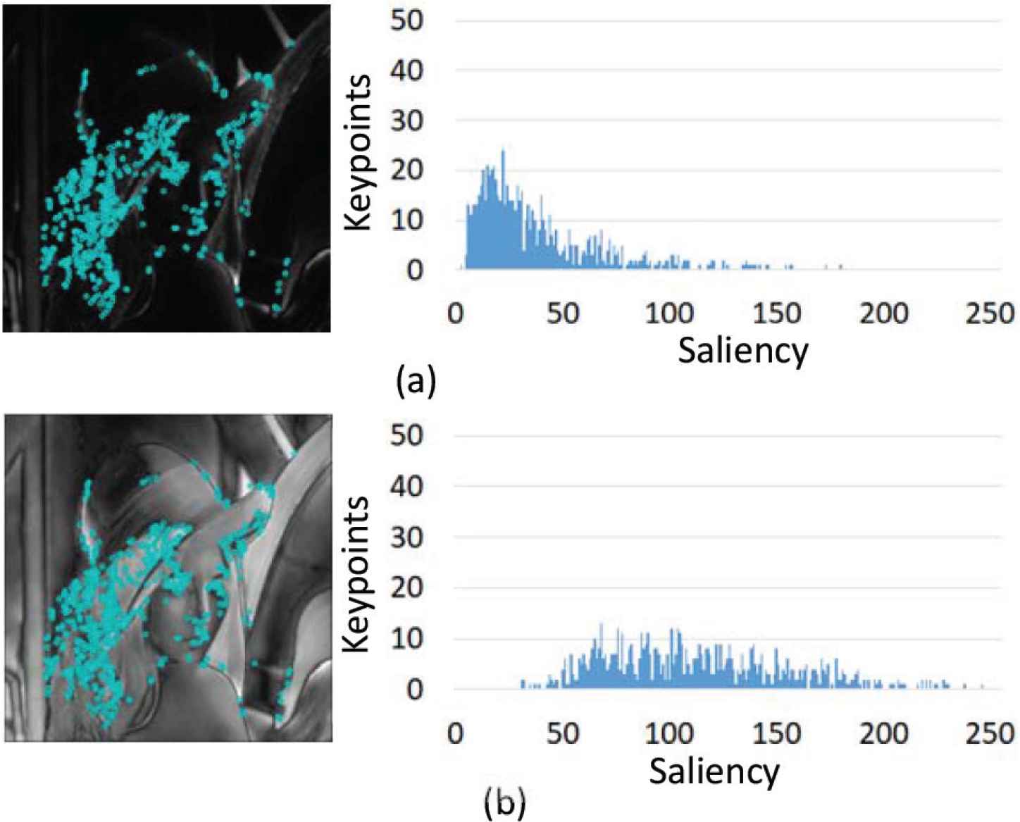
Keypoint location (Lenna). (a) Itti. (b) Proposed method (setting 2).
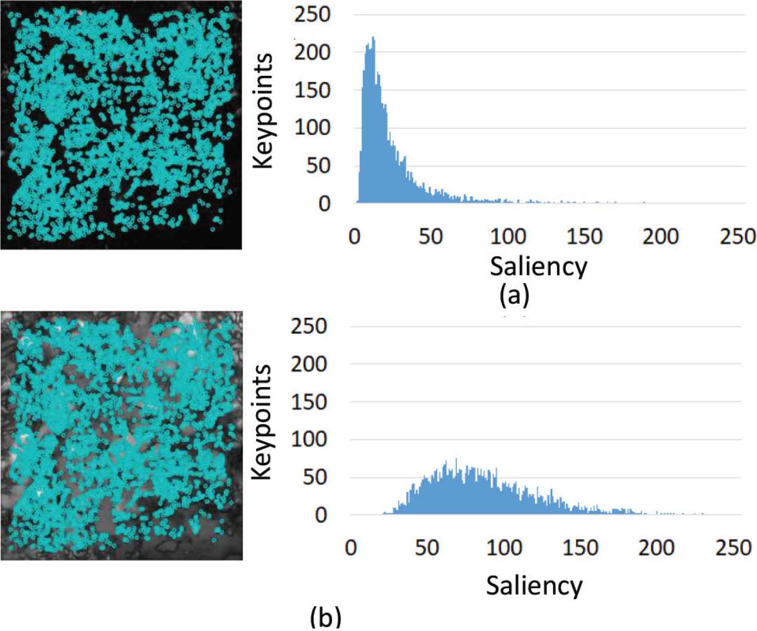
Keypoint location (Flower). (a) Itti. (b) Proposed method (setting 2).
5. CONCLUSION
In this research, we proposed method of saliency map generation which consists of adaptive filter adjustment to spatial frequency to aim at preventing fluctuation of saliency caused by different input image and photographing condition change. Our saliency map method turned to be suitable for selecting keypoints less affectable by photographing condition change compared with other conventional methods.
CONFLICTS OF INTEREST
The authors declare they have no conflicts of interest.
AUTHORS INTRODUCTION
Dr. Ryuugo Mochizuki
 He received his master of engineering degree at Kyushu Institute of Technology in 2008. Then he has been involved in spec test and design of Integrated Circuit as a worker in Shikino High-tech CO., LTD. up to 2013. His research topic during the doctor course was the relationship between scale-invariant keypoint extraction and saliency in the domain of image processing. He finished PhD degree in September 2019.
Dr. Kazuo Ishii
 He is a Professor in the Kyushu Institute of Technology, where he has been since 1996. He received his PhD degree in engineering from University of Tokyo, Tokyo, Japan, in 1996. His research interests span both ship marine engineering and Intelligent Mechanics. He holds five patents derived from his research. His lab got “Robo Cup 2011 Middle Size League Technical Challenge 1st Place” in 2011. He is a member of the Institute of Electrical and Electronics Engineers, the Japan Society of Mechanical Engineers, Robotics Society of Japan, the Society of Instrument and Control Engineers and so on.
REFERENCES
Cite this article
TY  - JOUR
AU  - Ryuugo Mochizuki
AU  - Kazuo Ishii
PY  - 2020
DA  - 2020/05/18
TI  - Evaluation of the Relationships between Saliency Maps and Keypoints
JO  - Journal of Robotics, Networking and Artificial Life
SP  - 16
EP  - 21
VL  - 7
IS  - 1
SN  - 2352-6386
UR  - https://doi.org/10.2991/jrnal.k.200512.004
DO  - 10.2991/jrnal.k.200512.004
ID  - Mochizuki2020
ER  -