
On Time Series Analysis for Repeated Surveys
Corresponding author. Email: mismail@feps.edu.eg
- DOI
- 10.2991/jsta.2018.17.4.1How to use a DOI?
- Keywords
- Cross section surveys; ARMA models; State space; Unemployment rate
- Abstract
Governments and other agencies repeated many important surveys at regular time intervals, but the population mean is estimated mainly using the latest survey. Time series estimators for the population mean using repeated surveys are superior to those obtained from the last survey. This superiority may be affected by several factors such as the sampling variance, the number of surveys, and the Auto Regressive Moving Average ARMA model coefficients and orders among others. The main objective of the paper is to compare the time series estimator for repeated surveys developed by Scott et al. (A.J. Scott, T.M.F. Smith, R.G. Jones, Int. Stat. Rev. 45 (1977), 13–28.) and the last survey estimator using extensive simulation studies. Furthermore, the impact of the factors that may affect the efficiency of the time series estimator is also investigated.
- Copyright
- © 2018 The Authors. Published by Atlantis Press SARL.
- Open Access
- This is an open access article under the CC BY-NC license (http://creativecommons.org/licences/by-nc/4.0/).
1. INTRODUCTION
Repeated surveys are usually used in economics and social science, by industry, government and research institutions to identify the characteristics of the population under study. It is often done at regular basis to monitor not only the level of some parameters of interest but also their changes in the intervals between surveys. It is also used to build up information on the trends of the phenomenon. The time series analysis for repeated surveys can be used to obtain more accurate estimation of the survey responses corresponding to the parameter of interest when compared to the traditional sample survey approach of separate parameter estimation at each time period (see [1]).
In Egypt, many surveys are repeated at fixed time intervals (monthly, quarterly, annually, or semiannually) such as labor force surveys conducted by the Egyptian Central Agency for Public Mobilization and Statistics (CAPMAS), and business surveys. Other surveys are repeated on an occasional basis. Examples include exit polls, and monitoring TV ratings. The time-series nature of these repeated surveys is seldom taken into account, which leads to lose the benefits of using the time series analysis of repeated surveys. The repeated nature of these surveys data creates a need for estimation procedures that combine information available from different times to produce the best estimates for the current mean or (percent estimators).
Using repeated surveys in estimating mean or percent of some indicators was subjected to many studies through the previous decades. Starting with Jessen [2], Patterson [3], Blight and Scott [4], Scott and Smith [5], Feder [6], Van den Brakel and Krieg [7], and many other studies tried to use different time series methods in repeated surveys. In Section 2, the literature of the time series methods used in repeated surveys is presented. A simulation study to compare between the last survey estimate and the time series estimator developed by Scott et al. [1] is provided in Section 3. In Section 4, an application of time series methods on the yearly Egyptian unemployment rate data obtained by the Egyptian CAPMAS (1980–2012) using the labor force survey is presented.
2. TIME SERIES ANALYSIS OF REPEATED SURVEYS
The time series repeated surveys estimators depend on the past information obtained from previous estimates to improve the current estimates. Time series repeated surveys estimators could have lower variance than the corresponding traditional estimators (see [8,9]). The improved time series repeated surveys estimators is no longer a function defined only on the sample at one time period t, but instead defined on all samples taken between two fixed time periods 1 and t. Thus, the estimator is derived from t periods of data. Previous studies on analyzing repeated survey methods can be classified into two categories; the classical method (non-stochastic approach), and the time series methods (stochastic approach).
The pioneer work of the classical methods was that of Jessen [2] for the sample of two occasions. Yates [10] extended Jessen's work for the case of constant sample size and a fixed replacement fraction on each occasion. Patterson [3] generalized the results of Jessen to the case of sampling on h occasions (surveys) with partial overlap of sampling units. Eckler [11] obtained a minimum variance estimate of the population value using the method of rotation sampling. Cochran [12] developed the optimum overlap for Patterson's [3] estimator when all samples are of equal size. Rao and Graham [13] used the rotations sample design to develop a unified finite population theory for composite estimators of the current levels. Singh [14] studied the effect of using multi-stage sample design on Patterson's estimator.
The time series approach can be a solution for problems of the classical methods in which any relationship between successive values of the population parameters is ignored completely, therefore using the classical methods requires the individual unit values be available to the analyst, however in many cases the individual units are not available for analysis, and the secondary analysis must be used, which in turn requires using the time series methods. For the time series methods, it can be classified into two categories; the ARMA method approach, and the state space approach.
Considerable interest has been shown in the methods of estimation for repeated surveys using time series analysis (ARMA method approach); Blight and Scott [4] discussed the effect of ignoring the relationship between successive values of the population parameters using a Bayesian approach. They also explored the effect of using such relationship in the estimation process.
Scott and Smith [5] used a more general approach than that used by Blight and Scott [4]. They assumed a stochastic model for the population means with a stationary process or a non-stationary process which can be reduced to a stationary form using differencing or subtracting deterministic components.
Scott et al. [1] extended the results of Scott and Smith [5] to surveys of complex designs, and applied their results on both overlapping and non-overlapping surveys. Some comparisons of Blight and Scott [4], Scott and Smith [5] approach with that of Patterson [3] using the mean square error (MSE) of the current mean was given by Jones [15]. Jones [16] derived a general form for the estimators derived by Blight and Scott [4], Scott and Smith [5], and Patterson [3] using the least square theory. The estimators of the population means obtained by Patterson, Blight and Scott, and Scott and Smith could be obtained from Jones's estimator using the generalized least square method. The problem of stationarity is also considered by Jones [16].
A new approach of the time series methods for repeated surveys is that of the state space approach. This approach consists of measurement, and transition equation. The population means are then estimated using the Kalman filter technique. Unlike the ARMA method approach, the state space approach can be useful in the cases where a small number of observations are used, or having a data with missing observations. Subsequent work for the state space approach by Tam [17], Rao et al. [18], Pfeffermann [19], Feder [6], Silva and Smith [20], Lind [21], Pfeffermann and Tiller [22], Sadik and Notodiputro [23], Van den Barkel and Krieg [24], and Krieg and Van den Barkel [25].
3. SIMULATION STUDY
3.1. Simulation Design
The simulation design in the current study is discussing two main cases:
Case 1: Correct specified time series models
Case 2: Miss-specified time series models
The sampling variance (S2)
The survey sampling errors were assumed to follow the normal distribution with zero mean and a sampling variance (S2), where the sampling variance takes the values 0.5, 1, or 2.
Number of surveys (t)
Different number of surveys t (the number of the sample means) were used to trace the efficiency of the following two estimators. The time series estimator obtained by Scott et al. [1] with the following equation:
And the last survey estimatorThe numbers of surveys used into the simulation are 10, 20, 50, and 100, where 10 represents smallest number of surveys and 100 represent the largest number of surveys.To check the effect of the series size, the selected number of surveys t was created using the last t values in the series of the sample means, so that the values for the sample means included in the smaller values for t, will be included in the larger values for t (if t = 20, then the sample means of the series of size 10 (t = 10) were included in the series).
The ARMA model coefficients
Different parameter values for the ARMA model coefficients (λθ and λe) were considered to investigate the effect of parameter uncertainty on the efficiency of the time series estimator (λ = 0, 0.2, 0.5, 0.7, or 0.9) for AR(1), and MA(1).
Based on the above design, we have all different scenarios given in Table 1.
| Scenario 1 | Scenario 2 | Scenario 3 | Scenario 4 | Scenario 5 | |||||||||||||||
|---|---|---|---|---|---|---|---|---|---|---|---|---|---|---|---|---|---|---|---|
| S2 | σ2 | t | S2 | σ2 | t | S2 | σ2 | t | S2 | σ2 | t | S2 | σ2 | t | |||||
| 0.5 | 0.5 | 10 | 0.5 | 0.5 | 10 | 0.5 | 0.5 | 10 | 0.5 | 0.5 | 10 | 0.5 | 0.5 | 10 | |||||
| 20 | 20 | 20 | 20 | 20 | |||||||||||||||
| 50 | 50 | 50 | 50 | 50 | |||||||||||||||
| 100 | 100 | 100 | 100 | 100 | |||||||||||||||
| 1 | 10 | 1 | 10 | 1 | 10 | 1 | 10 | 1 | 10 | ||||||||||
| 20 | 20 | 20 | 20 | 20 | |||||||||||||||
| 50 | 50 | 50 | 50 | 50 | |||||||||||||||
| 100 | 100 | 100 | 100 | 100 | |||||||||||||||
| 2 | 10 | 2 | 10 | 2 | 10 | 2 | 10 | 2 | 10 | ||||||||||
| 20 | 20 | 20 | 20 | 20 | |||||||||||||||
| 50 | 50 | 50 | 50 | 50 | |||||||||||||||
| 100 | 100 | 100 | 100 | 100 | |||||||||||||||
| 1 | 0.5 | 10 | 1 | 0.5 | 10 | 1 | 0.5 | 10 | 1 | 0.5 | 10 | 1 | 0.5 | 10 | |||||
| 20 | 20 | 20 | 20 | 20 | |||||||||||||||
| 50 | 50 | 50 | 50 | 50 | |||||||||||||||
| 100 | 100 | 100 | 100 | 100 | |||||||||||||||
| 1 | 10 | 1 | 10 | 1 | 10 | 1 | 10 | 1 | 10 | ||||||||||
| 20 | 20 | 20 | 20 | 20 | |||||||||||||||
| 50 | 50 | 50 | 50 | 50 | |||||||||||||||
| 100 | 100 | 100 | 100 | 100 | |||||||||||||||
| 2 | 10 | 2 | 10 | 2 | 10 | 2 | 10 | 2 | 10 | ||||||||||
| 20 | 20 | 20 | 20 | 20 | |||||||||||||||
| 50 | 50 | 50 | 50 | 50 | |||||||||||||||
| 100 | 100 | 100 | 100 | 100 | |||||||||||||||
| 2 | 0.5 | 10 | 2 | 0.5 | 10 | 2 | 0.5 | 10 | 2 | 0.5 | 10 | 2 | 0.5 | 10 | |||||
| 20 | 20 | 20 | 20 | 20 | |||||||||||||||
| 50 | 50 | 50 | 50 | 50 | |||||||||||||||
| 100 | 100 | 100 | 100 | 100 | |||||||||||||||
| 1 | 10 | 1 | 10 | 1 | 10 | 1 | 10 | 1 | 10 | ||||||||||
| 20 | 20 | 20 | 20 | 20 | |||||||||||||||
| 50 | 50 | 50 | 50 | 50 | |||||||||||||||
| 100 | 100 | 100 | 100 | 100 | |||||||||||||||
| 2 | 10 | 2 | 10 | 2 | 10 | 2 | 10 | 2 | 10 | ||||||||||
| 20 | 20 | 20 | 20 | 20 | |||||||||||||||
| 50 | 50 | 50 | 50 | 50 | |||||||||||||||
| 100 | 100 | 100 | 100 | 100 | |||||||||||||||
The different scenarios for the simulation design.
3.2. Simulation Steps
Data is generated from ARMA (p, q) where 600 random values for the random error ϵt are firstly generated assuming that ϵtN(0, σ2), where the variance takes the values 0.5, 1, or 2.
The pseudo population means θt were created assuming that the initial values are zeroes.
The first 500 values of the series are deleted to remove the initialization effect. For each of the factors mentioned in Table 1, the process is repeated 10 000 runs, and for every run the values of the two estimators; Eqs. (1) and (2) are recorded.
The MSEs and the confidence intervals for the two estimators are then computed to compare the efficiency of the two estimators.
The MSE is computed as averages across all other factors, for example to compute the MSE for S2 = 0.5, we get the averages over all cases of t and λ
3.3. Simulation Results
The results for the comparisons for the two estimators are presented first for the two cases (correct specified, and miss-specified) as an overall result, then the comparison is done for each of the factors described in Table 1.
3.3.1. The Overall Results
Correct Specified Time Series Models
Figure 1 displays the boxplot for the MSE of the two estimators using different time series models.
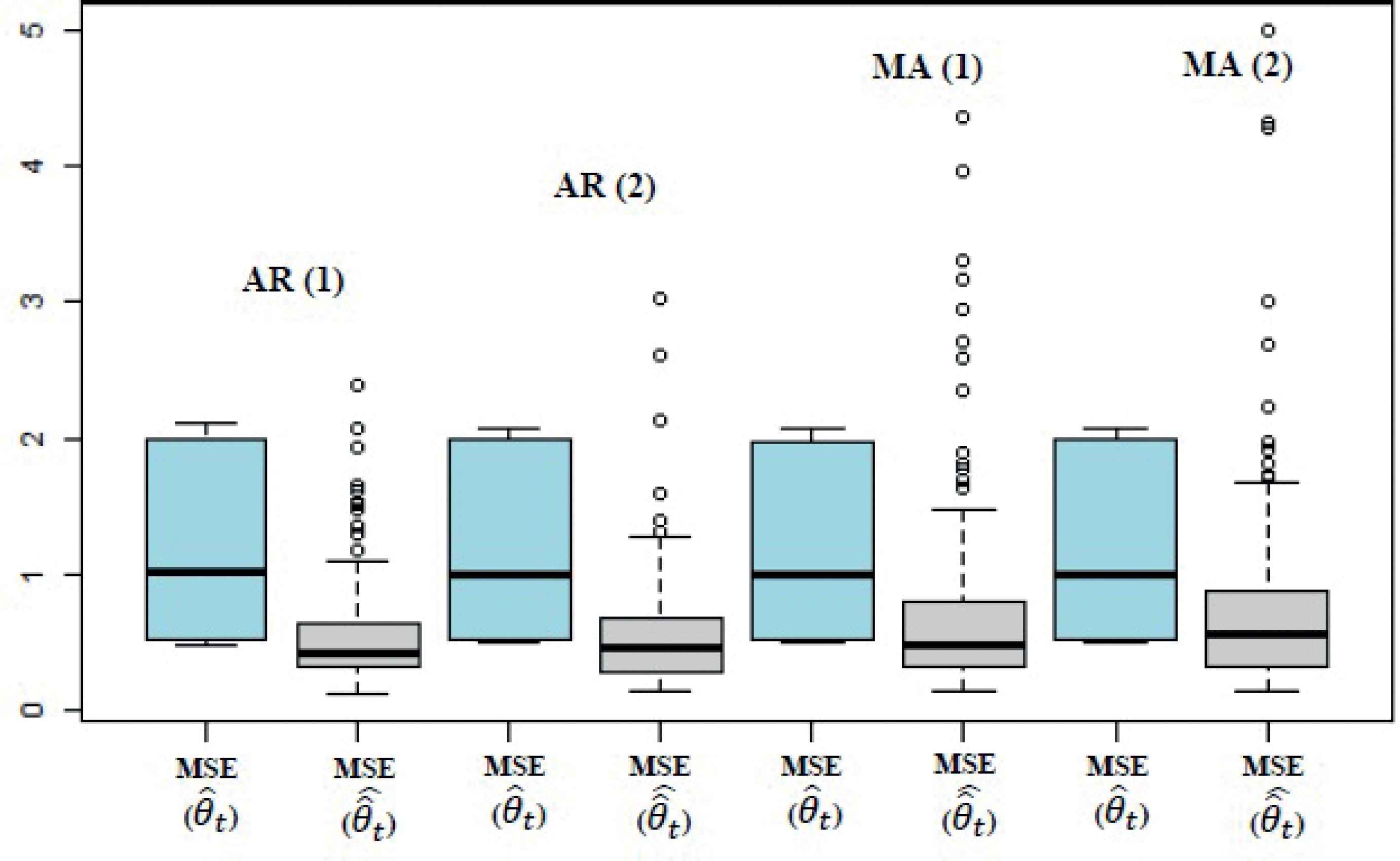
The box plot for the MSE of the two estimators using the different time series models.
Based on Fig. 1, it can be noticed that the 1st quartile, the median, and the 3rd quartile of the MSE of the time series estimators are always less than those of the last survey estimator using the different Time Series Modeling TSM, which indicates the superiority of the time series estimator when compared to the last survey estimator.
Also, the boxplots of the time series estimator are taller than that of the last survey estimator as 50% of the MSE of the time series estimators are between 0.30 and 0.64 for AR(1), 0.28 and 0.68 for AR(2), 0.32 and 0.80 for MA(1), and 0.32, and 0.87 for MA(2) whereas 100% of the MSE of the last survey estimator are around 0.5 and 2 for the different time series models (this is logically true as the MSE of the last survey estimator is the same as the sampling variance S2, and that may indicate that the simulation is correctly implemented). From Fig. 1, we conclude that the values of the MSE of the time series estimator are more homogeneous than that of the last survey estimator, and they are centered on small values of the MSE which reflects the efficiency of the time series estimator.
Miss-specified Time Series Models
Table 2 displays the MSE for the last and time series estimators using the different miss-specified time series models.
| Model | AR(1) Diff | AR(2) Diff | MA(1) Diff | MA(2) Diff |
|---|---|---|---|---|
| AR(1) | −0 58 | −0.78 | −0.33 | −0.36 |
| AR(2) | −0.67 | −0.60 | −0.43 | −0.51 |
| MA(1) | −0.75 | −0.64 | −0.46 | −0.63 |
| MA(2) | −0.56 | −0.57 | −0.44 | −0.42 |
The average difference between the MSE for the last estimator and time series estimators using different TSM.
The comparison between the MSEs for the two estimators indicates that the MSE of
3.3.2. Results Based on Simulation Factors for Correct Specification Case
Sampling Variance (S2)
First to be investigated is the sampling variance S2. The results show that the values of the MSE of the time series and last survey estimators get larger when the sampling variance is larger. The superiority of
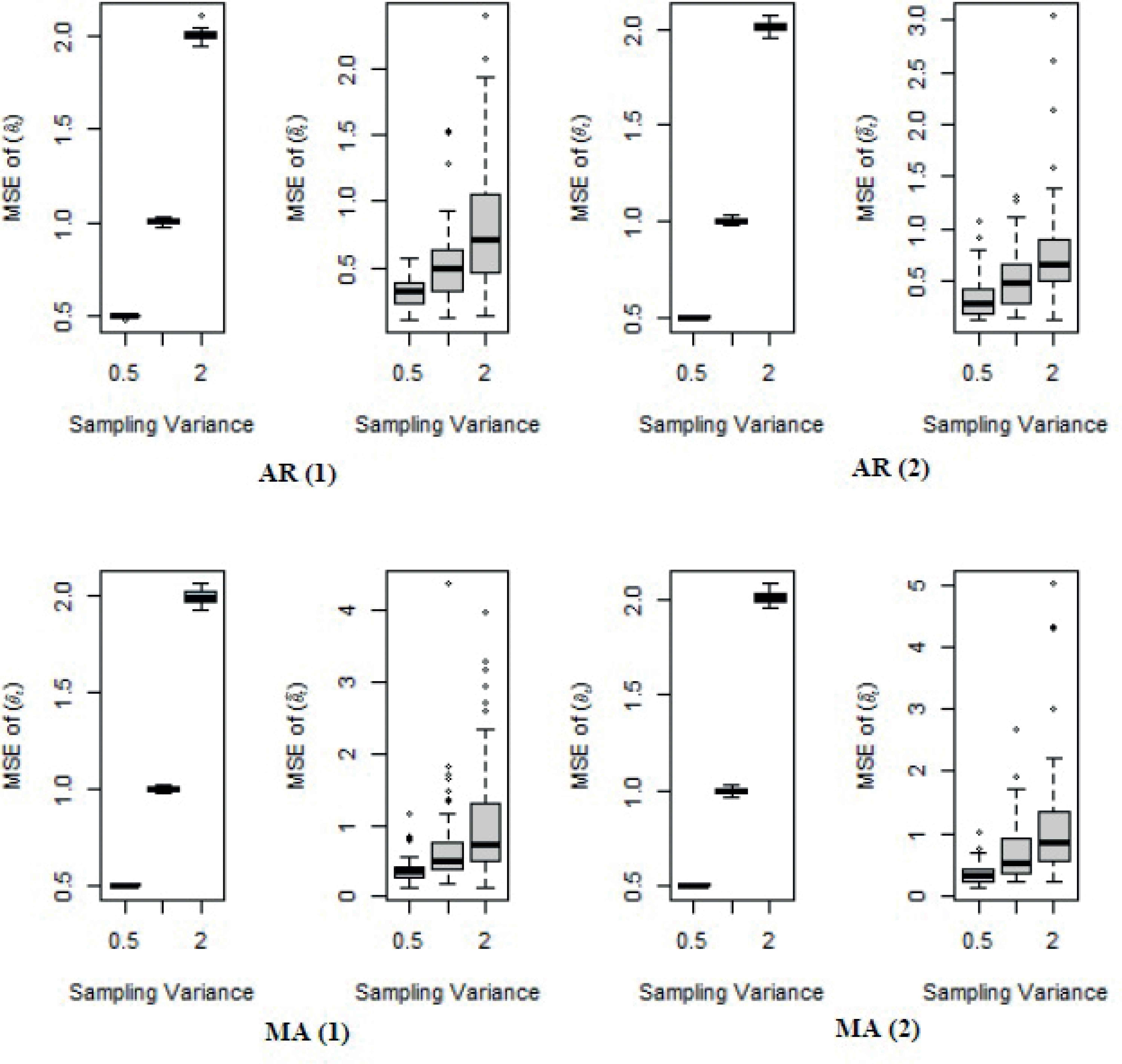
The MSE for the last and time series estimators using the different correct TSM according to the sampling variance.
It seems from the boxplots that the MSEs of the last survey estimator are always around the values of the sampling variance (S2) which provides an evidence for the validity of the simulation (the MSE of the last survey estimator is supposed to equal to the sampling variance (S2)). It can also be found that the 1st quartile, the median, and the 3rd quartile, of the MSE of the time series estimators are always less than those of the last survey estimator for all different values of the sampling variance (S2).
The Number of Surveys (t)
The second factor is the number of surveys (t). It is clear that the superiority of

The MSE for the last and time series estimators using different correct TSM according to the number of surveys.
Figure 3 shows that the median of the MSE of the time series estimator nearly decreases when using larger values for the number of surveys (t). It is also found that the first quartile, the median and the third quartile of the MSE of the time series estimator are always less than those of the last survey estimator for the different values of (t). When using MA(1) model, it was found that the median of the MSE of the last survey estimator is less than that of the time series estimator when the number of surveys (t = 10). This implies that the time series estimator may suffer from the problem of model failure when using a small number of surveys as was indicated in the literature, see e.g., Tam [17].
The Model Coefficient (λ)
The analysis of the results according to the value of λ doesn't detect any clear pattern for the relation between the MSE of
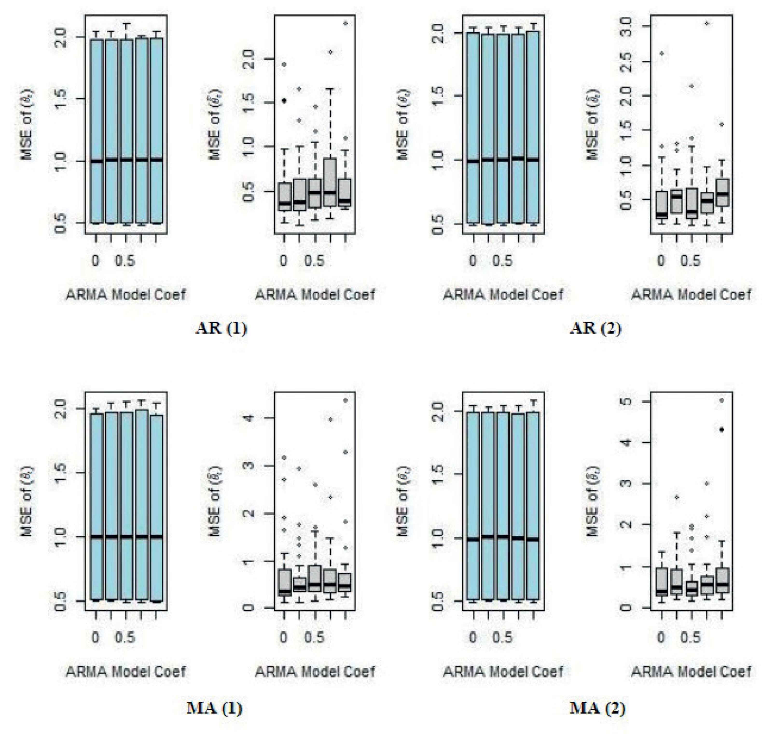
The MSE for the last and time series estimators using the different TSM according to ARMA model coefficients.
As shown in Fig. 4, the 1st quartile, the median and the 3rd quartile of the time series estimator are always less than those of the last survey estimator using the different time series models, which reflects the superiority of the time series estimator. However, the values of the MSE of the time series estimator haven't any clear pattern for the different values of λ.
3.3.3. Results Based on Simulation Factors for Miss-specified Case
Sampling Variance (S2)
For the case of miss-specified time series models, the MSE of
As shown from Table 3, the difference between the MSE of the last survey and the time series estimators using the miss-specified AR(2) instead of the correct AR(1) still increases with S2 and reaches −1.44 for S2 = 2 which is larger than the difference when S2 = 0.5 and 1 (the difference = −0.26, and −0.66 respectively). Similar results can be found when using the other miss-specified models for AR(1) or the other miss-specified models for AR(2), MA(1), and MA(2).
| Model | S2 | AR(1) Diff | AR(2) Diff | MA(1) Diff | MA(2) Diff |
|---|---|---|---|---|---|
| AR(1) | 0.5 | −0.18 | −0.26 | −0.12 | −0.11 |
| 1.0 | −0.48 | −0.66 | −0.27 | −0.24 | |
| 2.0 | −1.14 | −1.44 | −0.63 | −0.73 | |
| AR(2) | 0.5 | −0.18 | −0.15 | −0.14 | −0.16 |
| 1.0 | −0.51 | −0.46 | −0.34 | −0.36 | |
| 2.0 | −1.34 | −1.21 | −0.84 | −1.04 | |
| MA(1) | 0.5 | −0.22 | −0.14 | −0.14 | −0.22 |
| 1.0 | −0.60 | −0.47 | −0.30 | −0.57 | |
| 2.0 | −1.43 | −1.41 | −0.94 | −1.11 | |
| MA(2) | 0.5 | −0.18 | −0.26 | −0.12 | −0.11 |
| 1.0 | −0.16 | −0.22 | −0.16 | −0.14 | |
| 2.0 | −1.14 | −1.09 | −0.80 | −0.83 |
All bolded numbers are significant at 0.05
The average difference between the MSE of
The Number of Surveys (t)
Under the miss-specification case, the superiority
| Model | S2 | AR(1) | AR(2) | MA(1) | MA(2) |
|---|---|---|---|---|---|
| Diff | Diff | Diff | Diff | ||
| AR(1) | 10 | −0.26 | -.- | −0.32 | -.- |
| 20 | −0.48 | −0.72 | −0.58 | −0.06 | |
| 50 | −0.63 | −0.84 | −0.50 | −0.51 | |
| 100 | −0.71 | −0.78 | −0.51 | −0.49 | |
| AR(2) | 10 | −0.21 | -.- | −0.50 | -.- |
| 20 | −0.60 | −0.52 | −0.62 | −0.38 | |
| 50 | −0.76 | −0.63 | −0.73 | −0.51 | |
| 100 | −0.71 | −0.65 | −0.74 | −0.64 | |
| MA(1) | 10 | -.- | -.- | −0.50 | -.- |
| 20 | −0.64 | −0.23 | −0.43 | −0.33 | |
| 50 | −0.83 | −0.71 | −0.69 | −0.81 | |
| 100 | −0.78 | −0.78 | −0.71 | −0.78 | |
| AR(1) | 10 | −0.19 | -.- | −0.31 | −0.10 |
| 20 | −0.53 | −0.29 | −0.58 | −0.12 | |
| 50 | −0.72 | −0.65 | −0.78 | −0.51 | |
| 100 | −0.56 | −0.65 | −0.62 | −0.63 |
All bolded numbers are significant at 0.05
The average difference between the MSE of
From Table 4, there is a slight increase in the difference between the MSE of the last survey and time series estimators when using larger values of t even if using miss-specified TSM. However, when using small number of surveys and miss-specified TSM, the efficiency of the time series estimator gets lower compared to that of the last survey estimator. The difference becomes 0.32, 0.5, and 0.31 when using the miss-specified MA(1) for the correct AR(1), AR(2), and MA(2), respectively. (The time series estimator suffers from the problem of model failure as mentioned in the literature.)
4. THE ANNUAL UNEMPLOYMENT RATE
Our two estimators are applied for the series of the annual unemployment rate. This series ran from the period of 1980 until the end of the year 2012.1 The source of the data is the Egyptian Labor Force Surveys conducted by the Egyptian CAPMAS. This survey was first conducted in November 1957, and since then the survey has been conducted but in irregular periodicity as it was conducted annually in times and biannually or quarterly in others. It aims at measuring the Egyptian civilian labor force and its characteristics, measuring the level of employment in different geographic areas of the republic, and measuring the geographic distribution of the employed population according to many characteristics like gender, age, education, etc. The survey sample is a two-stage stratified cluster sample, and its size is about 21 352 households for each round allocated among governorates and their urban/rural components in proportion to size (Fig. 5).
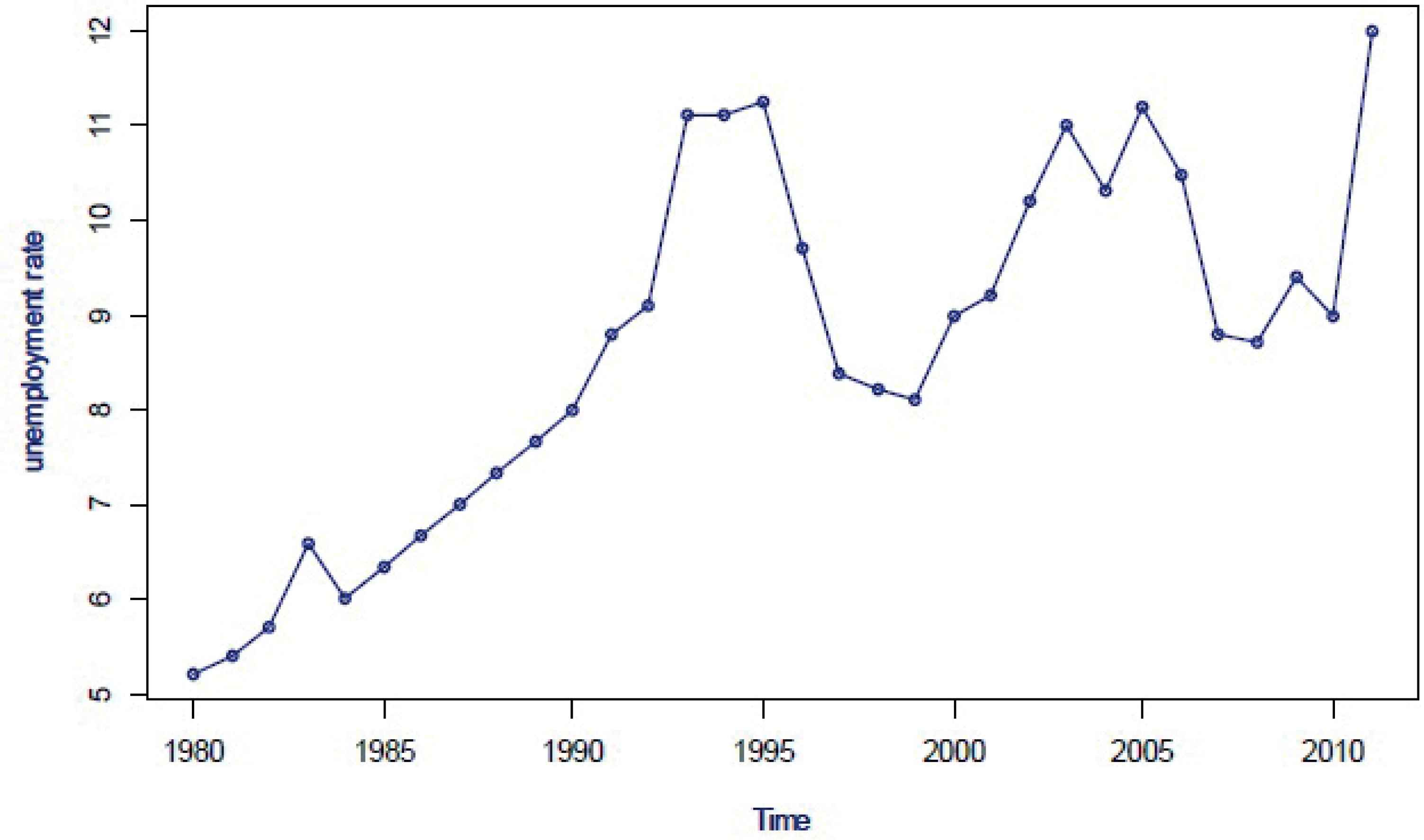
The time series plot for the Egyptian unemployment rate during the period 1980–2012.
Following Box and Jenkins procedures to estimate the model for the yearly unemployment rate resulted in an ARIMA (1,2,1) model. This model achieved all the assumptions and seems to be efficient to represent the data. Hence the estimated values for π and
| The factor | The estimated value |
|---|---|
| 1.510 | |
| S2 | 1.005 |
| π | 0.666 |
| 12.700 | |
| 12.966 |
Comparison of acoustic for frequencies for piston-cylinder problem.
The unemployment rate in 2012 records 13% using the time series estimator compared to 12.7% using the last survey estimator as shown in Table 1. This represents only 0.3% underestimation of the value of the unemployed people reached by the labor force survey. The gains due to the time series method depend on the value of
A 95% confidence intervals for the mean of the unemployment rate of
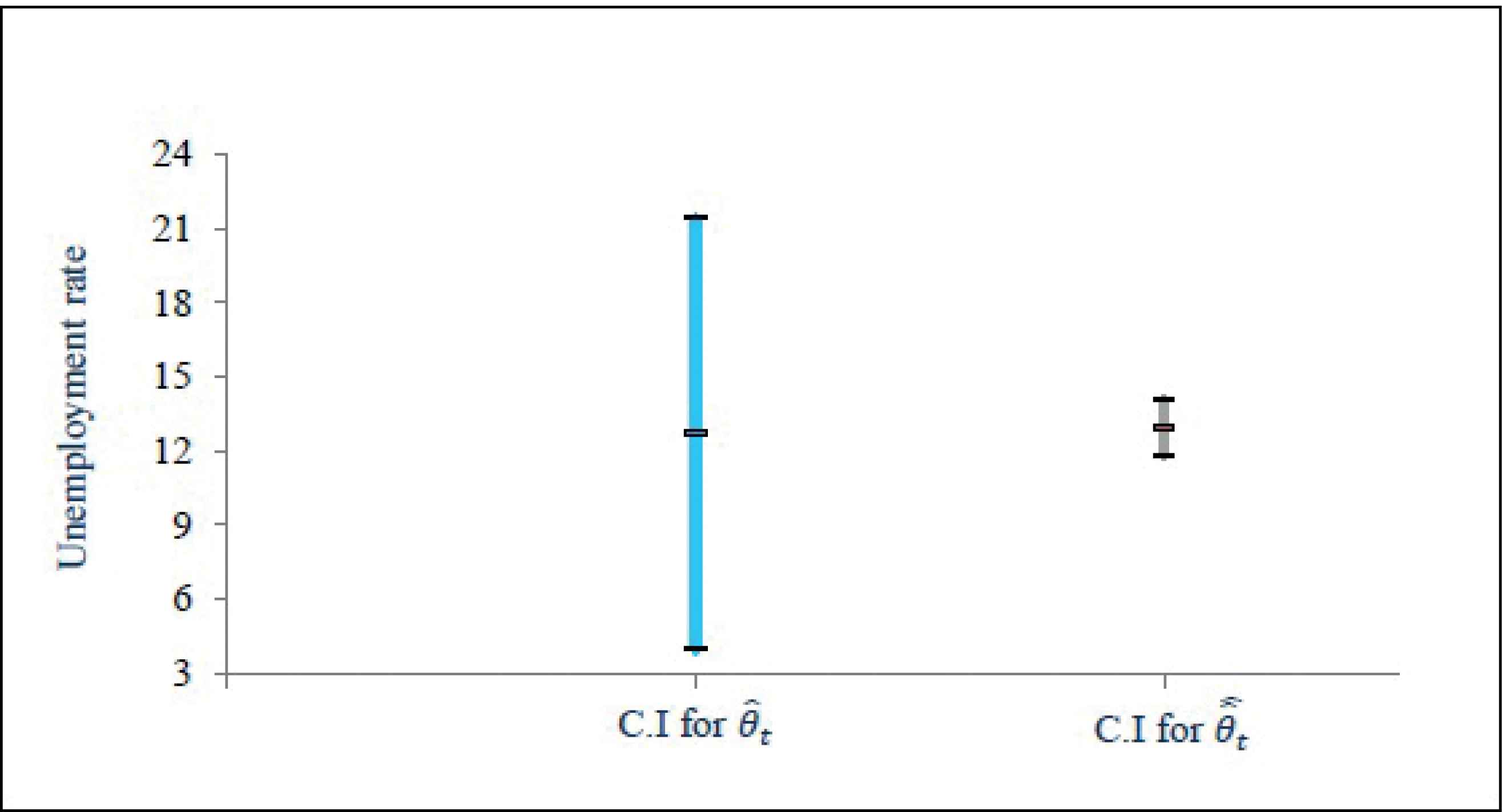
A 95% confidence interval for the time series and last survey estimators using the unemployment rate.
5. CONCLUSION
The analysis of repeated surveys using time series methods is seldom taken into account. The estimation of the mean of the phenomena usually depends on the last survey, although it is more efficient to use the time series analysis in the estimation process as the time series for repeated surveys estimators could have lower variance than the corresponding traditional estimators. This was confirmed using the simulation study which indicated that the MSE of the time series mean
It is shown from the current study that the values of the 2 MSE's get larger when the sampling variance is larger, and also the superiority of
CONFLICT OF INTEREST
Interest time series analysis & repeated surveys
Footnotes
The data during the period 1985 until 1989 were missing, and they were replaced using the linear interpolation method.
REFERENCES
Cite this article
TY  - JOUR
AU  - Mohamed A. Ismail
AU  - Hend A. Auda
AU  - Yehia Ahmed Elzafrany
PY  - 2018
DA  - 2018/12/31
TI  - On Time Series Analysis for Repeated Surveys
JO  - Journal of Statistical Theory and Applications
SP  - 587
EP  - 596
VL  - 17
IS  - 4
SN  - 2214-1766
UR  - https://doi.org/10.2991/jsta.2018.17.4.1
DO  - 10.2991/jsta.2018.17.4.1
ID  - Ismail2018
ER  -