
Weibull-Normal Distribution and its Applications
Corresponding author. Email: felix.famoye@cmich.edu
- DOI
- 10.2991/jsta.2018.17.4.12How to use a DOI?
- Keywords
- T-R{Y} framework; Bimodal; Hazard function; Estimation
- Abstract
In this paper, a Weibull-normal distribution, based on the standard quantile function of log-logistic distribution, is defined and studied. Some properties of the probability distribution are discussed. The Weibull-normal distribution is found to be unimodal or bimodal. The distribution can be right skewed or left skewed. The method of maximum likelihood estimation is suggested to estimate the parameters of the distribution. Three numerical data sets are used to illustrate the applications of the Weibull-normal distribution.
- Copyright
- © 2018 The Authors. Published by Atlantis Press SARL.
- Open Access
- This is an open access article under the CC BY-NC license (http://creativecommons.org/licences/by-nc/4.0/).
1. INTRODUCTION
The theory of statistical distributions continues to be a strong area of research. A lot has been done on the univariate distributions and in particular, the continuous univariate distributions. For a review of methods of generating statistical distributions in the recent decades, the reader is referred to Ref. [1]. In this reference, a chronological reference to how the beta-generated family, the Kumaraswamy generated (Kum-generated for short) family and the generalized beta-generated family led to the T-X family of distributions. Subsequently, we have the T-R{Y} family introduced by Ref. [2], with a unified notation provided in Ref. [3].
The beta-generated family of distributions was introduced by Ref. [4]. The cumulative distribution function (CDF) of the family is given by
The beta-generated family of distributions was extended (Refs. [6] and [7]) to the Kumaraswamy-generated family of distributions by replacing the beta distribution with Kumaraswamy distribution. The PDF of the Kumaraswamy distribution (Ref. [8]) is given by
The T-X(W) family of distributions, which extended the beta-generated, Kumaraswamy-generated, and generalized beta-generated families, was introduced by Ref. [10]. The CDF of the family is given by
In Section 2, we define the Weibull-normal{log-logistic} distribution. In Section 3, we provide some properties, including the modes and the Shannon entropy. The method of maximum likelihood estimation is proposed for estimating the distribution parameters in Section 4. A simulation study in Section 5 is used to evaluate the performance of the maximum likelihood estimation method. In Section 6, we illustrate the applications of the distribution with three numerical real life data sets and the results are compared with other distributions. We provide a summary in Section 7.
2. WEIBULL-NORMAL{LOG-LOGISTIC} DISTRIBUTION
Suppose a random variable T follows the Weibull distribution with parameters c and γ. Then, the CDF of T is given by
For the log-logistic distribution, the quantile function is given by
The hazard function of the W-N{LL} is given by
2.1. Limits of the PDF and Hazard Function of the W-N{LL}
As
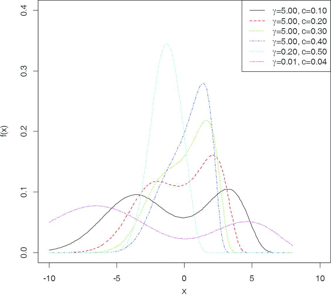
PDFs of W-N{LL} for µ = 0 and σ = 1 for various values of c and γ.
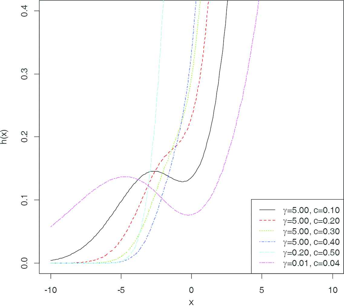
Hazard functions of W-N{LL} for µ = 0 and σ = 1 for various values of c and γ.
2.2. Quantile Function
To find the quantile function of W-N{LL}, we solve the equation
The median of the W-N{LL} is given by
3. SOME PROPERTIES OF WEIBULL-NORMAL{LOG-LOGISTIC} DISTRIBUTION
In this section, we provide some properties of the W-N{LL} distribution.
3.1. Transformations
Lemma 1.
If X follows a W-N{LL} distribution with parameters c, γ, µ and σ, then the random variable
Proof. By using the transformation method, the result follows.
The above lemma can be used to transform the W-N{LL} random variate X into a Weibull random variate Y. For example, the starting values for the parameters c, γ, µ and σ in a W-N{LL} can be obtained by using the moment estimates for normal and Weibull random variates. The W-N{LL} is a generalization of the normal distribution. Take the variate as normal random variate and compute the sample mean and sample standard deviation as the initial estimates of µ and σ respectively. Use Lemma 1 to transform the variate X into Y, a Weibull random variate. Then obtain the initial estimates of c and γ as the corresponding moment estimates.
Lemma 2.
Suppose Y has a standard exponential distribution. Suppose X has a normal distribution with mean µ and standard deviation σ such that
Proof. Use the transformation method.
Lemma 3.
Suppose Y has a Pareto distribution with CDF
Proof. Use the transformation method.
Lemma 4.
Suppose Y has a Fréchet distribution with CDF
Proof. Use the transformation method.
Lemma 5.
Suppose Y has a Gumbel distribution with CDF
Proof: Use the transformation method.
3.2. Modes of W-N{LL} Distribution
The mode(s) of the W-N{LL} distribution is given by equating to zero the derivative with respect to x of the PDF
When c

Unimodal and bimodal regions of W-N{LL} distribution.
When 0.119
3.3. Shannon Entropy
The Shannon entropy of a random variable X is a measure of variation of uncertainty. It is defined by Ref. [11] as
3.4. Mean Deviation about the Mean μ
The mean deviation about the population mean and population median are given by Ref. [3], and these are not provided here.
4. ESTIMATION OF W-N{LL} DISTRIBUTION PARAMETERS
Suppose we have a random sample of size n from the W-N{LL} distribution with parameters c, γ, µ and σ. The likelihood function is given as
One can obtain the second partial derivatives and these can be used to find the variance-covariance matrix for the parameter estimates. The equations in (7) through (10) are solved by an iterative technique to obtain the maximum likelihood estimates
5. SIMULATION
In order to evaluate the performance of the maximum likelihood estimation method, we conduct a simulation study. The quantile function in Eq. (5) is used to generate a random sample from the Weibull-normal{log-logistic} distribution with parameters c, γ, µ and σ. The parameters α and σ are fixed at α = 4 and σ = 2 for the whole simulation study. The parameter combinations for c and σ are varied and they are given in Table 1. The combinations are selected to reflect when the distribution is bimodal and unimodal. The case where c = 0.2 and γ = 2, 4, and 6 represent bimodal cases while c = 0.5 and γ = 2, 4, and 6 represent unimodal cases. For each parameter combination and each sample size, the simulation process is repeated 200 times. The average bias (actual – estimate) and the standard deviation of the parameter estimates are reported in Table 1. The biases are relatively small when compared to the standard deviations. In most cases, as the sample size increases, the standard deviations of the estimators decrease.
| Actual values | Bias with standard deviation in parentheses | |||||
|---|---|---|---|---|---|---|
| n | c | γ | ||||
| 250 | 0.2 | 2.0 | −0.006(0.036) | 0.062(0.434) | −0.018(0.268) | −0.036(0.235) |
| 0.2 | 4.0 | −0.006(0.037) | 0.168(0.920) | −0.029(0.253) | −0.021(0.235) | |
| 0.2 | 6.0 | 0.003(0.035) | 0.486(1.292) | 0.012(0.301) | 0.023(0.227) | |
| 0.5 | 2.0 | 0.009(0.102) | 0.077(0.428) | −0.060(0.263) | 0.033(0.335) | |
| 0.5 | 4.0 | 0.020(0.092) | 0.045(0.895) | −0.098(0.311) | 0.075(0.282) | |
| 0.5 | 6.0 | 0.006(0.094) | 0.073(1.333) | −0.081(0.384) | 0.040(0.294) | |
| 500 | 0.2 | 2.0 | −0.004(0.032) | 0.043(0.435) | −0.015(0.208) | −0.019(0.209) |
| 0.2 | 4.0 | −0.002(0.030) | 0.204(0.855) | −0.042(0.208) | −0.007(0.186) | |
| 0.2 | 6.0 | 0.001(0.030) | 0.428(1.275) | −0.013(0.199) | 0.012(0.191) | |
| 0.5 | 2.0 | 0.002(0.088) | 0.046(0.412) | −0.059(0.230) | 0.011(0.282) | |
| 0.5 | 4.0 | −0.005(0.084) | 0.093(0.892) | −0.052(0.283) | −0.011(0.273) | |
| 0.5 | 6.0 | −0.003(0.085) | 0.148(1.388) | −0.047(0.300) | −0.006(0.263) | |
| 750 | 0.2 | 2.0 | −0.004(0.030) | 0.073(0.410) | −0.031(0.181) | −0.021(0.197) |
| 0.2 | 4.0 | −0.001(0.027) | 0.099(0.854) | −0.035(0.194) | 0.002(0.169) | |
| 0.2 | 6.0 | −0.003(0.028) | 0.544(1.317) | −0.033(0.182) | −0.015(0.177) | |
| 0.5 | 2.0 | −0.009(0.081) | 0.059(0.389) | −0.058(0.225) | −0.024(0.259) | |
| 0.5 | 4.0 | 0.003(0.074) | 0.032(0.821) | −0.038(0.226) | 0.009(0.229) | |
| 0.5 | 6.0 | −0.010(0.070) | 0.183(1.243) | −0.044(0.238) | −0.020(0.215) | |
Bias and standard deviation of maximum likelihood estimates when α = 4 and σ = 2.
6. APPLICATIONS
In this section, the W-N{LL} distribution is applied to three data sets and the results are compared with other distributions.
6.1. Amount of Money Paid to Insurance Policy Holders
The data analyzed in this sub-section is the amount of money paid by an insurance company in Nigeria to policy holders when they discontinue and ‘drop out’. The data consists of a random sample of 195 customers and the data is available from the second author. The logarithm of the amount paid is fitted by using the Weibull-normal{log-logistic} distribution, the BN distribution defined and studied by Ref. [4], and Cauchy-Weibull{logistic} (C-W{L}) distribution defined and studied by Ref. [13]. The data is skewed to the right (skewness = 0.2574 and kurtosis = –0.5231). The results from the three distributions are presented in Table 2. The Akaike Information Criterion (AIC) and the Kolmogorov-Smirnov (KS) goodness of fit statistic with its corresponding p-value are reported in Table 2. From the table, both the W-N{LL} and BN distributions provide adequate fit to the data set while the C-W{L} distribution does not provide a good fit to the data.
| Distribution | C-W{L} | BN | W-N{LL} |
|---|---|---|---|
| Parameter estimates | |||
| Log-likelihood | −364.00 | −341.63 | −341.75 |
| AIC | 736.0 | 691.3 | 691.5 |
| KS statistic (p-value) | 0.1225 (0.0057) | 0.0480 (0.7606) | 0.0504 (0.7042) |
Parameter estimates (standard errors) for insurance policy holders data.
6.2. USS Halfbeak Engine Data
The USS Halfbeak diesel engine data was used by Ref. [14] to illustrate the application of McDonald-gamma (Mc-G) distribution. The distribution of the data is highly skewed to the left and it is platykurtic (skewness = –1.5764 and kurtosis = 1.6525). Ref. [2] also fitted the data to a four-parameter normal-Weibull{Cauchy} (N-W{C}) distribution. The fits from N-W{C} and Mc-G distributions are obtained from Ref. [2] and are given in Table 3. In Table 3, we provide the parameter estimates and the goodness of fit statistics. Only two of the three distributions in Table 3 provide adequate fit to the data set. Furthermore, both N-W{C} and W-N{LL} provide almost identical fit to the data when we consider both the log-likelihood and the AIC statistics.
| Distribution | Mc_G* | N-W{C}* | W-N{LL} |
|---|---|---|---|
| Parameter estimates | |||
| Log-likelihood | −217.35 | −196.45 | −196.18 |
| AIC | 444.7 | 400.9 | 400.4 |
| KS statistic (p-value) | 0.2635 (1.045E-04) | 0.0811 (0.739) | 0.0895 (0.6200) |
Estimates from Ref. [2]
Parameter estimates (standard errors) for the USS Halfbeak diesel engine data.
6.3. Crops Produce Data
The data analyzed in this sub-section are the prices of some crops produced in Nigeria. The variable is the farmgate price in Naira (Nigeria monetary unit) per kilogram of crops obtained from Nigeria National Bureau of Statistics. The variable is the addition of farmgate prices for the following 13 crops produce: cowpea, cassava, maize, cocoyam, groundnut, rice, yam, rice, melon, soybeans, sesame seed and palm oil. The data was collected for 2006 through 2015 for each of the 36 states in Nigeria and the Federal Capital Territory (Abuja) leading to n = 37 data points for each year. For this analysis, we used the data for 2015, the most recent year that has data available (the data is available from the third author). The data is negatively skewed (skewness = –0.3010 and kurtosis = –0.7214)
We applied the four-parameter BN distribution by Ref. [4], the four-parameter normal-Weibull{Cauchy} (N-W{C}) distribution by Ref. [2] and the W-N{LL} distribution defined and studied in this paper to analyze the data. The results of the fits are provided in Table 4. All the three distributions provide adequate fit to the data. However, the W-N{LL} distribution provides the best K-S statistic and has a slightly smaller AIC value than the other two distributions.
| Distribution | BN | N-W{C} | W-N{LL} |
|---|---|---|---|
| Parameter estimates | |||
| Log-likelihood | −180.06 | −180.38 | −179.36 |
| AIC | 368.1 | 368.8 | 366.7 |
| KS statistic (p-value) | 0.1141 (0.7207) | 0.1056 (0.8037) | 0.0617 (0.9989) |
Parameter estimates (standard errors) for the crops produce data.
7. SUMMARY
A new generalization of the normal distribution is defined and studied. The Weibull-normal{log-logistic} (W-N{LL}) distribution can be skewed to the left or skewed to the right. The distribution can be unimodal or bimodal. When the shape parameter c = 1, the W-N{LL} distribution reduces to the exponential-normal{log-logistic} distribution with three parameters. This special case is always unimodal since the shape parameter c is set to 1. The method of maximum likelihood estimation is proposed for estimating the parameters of W-N{LL} distribution. The distribution is applied to three data sets and it is found to perform well in fitting the data sets compared to other distributions. From the data sets in Section 6, we notice that the W-N{LL} distribution is capable of providing adequate fit to data sets that are about symmetric or skewed to the left or skewed to the right.
ACKNOWLEDGEMENT
The first author gratefully acknowledges the financial support received from the U.S. Department of State, Bureau of Education and Cultural Affairs under the Fulbright Grant # PS00230565.
REFERENCES
Cite this article
TY  - JOUR
AU  - Felix Famoye
AU  - Eno Akarawak
AU  - Matthew Ekum
PY  - 2018
DA  - 2018/12/31
TI  - Weibull-Normal Distribution and its Applications
JO  - Journal of Statistical Theory and Applications
SP  - 719
EP  - 727
VL  - 17
IS  - 4
SN  - 2214-1766
UR  - https://doi.org/10.2991/jsta.2018.17.4.12
DO  - 10.2991/jsta.2018.17.4.12
ID  - Famoye2018
ER  -