1. INTRODUCTION

Astronomical data, coming from different sources and collected by different telescopes, are often needed to be combined in a complete data set for study. In this situation, it is always very important to test compatibility of two data sets, collected in different surveys or measured with different resolutions, before pooling them together and they can only be combined when they are compatible (see, e.g., [1,2]). That means, they should have approximately the same amount of observational error on an average. One possible way to deal with this situation is to carry out the following hypothesis testing problem under multivariate set up:

Let X1,…,Xn1 and Y1,…,Yn2 be two independent samples from p–variate p≥2 populations with continuous distribution functions (d.f.s) F and G respectively, where Gx=Fx−Δ for all x∈Rp. We consider the problem of testing the null hypothesis H0:Δ=0 against the alternative H1:Δ≠0. Our test can be employed to solve the above stated problem and indicates compatibility only when the null hypothesis is accepted.

In this context, the Hotelling T2 test HT is optimal and unbiased when F is a p–variate normal d.f. However, for non-normal population, its finite sample unbiasedness is not certain [3]. It performs poorly for high-dimensional data [4] and the observations affected by outliers. Moreover, it is incomputable when p>n1+n2−2. In astronomy, data collection on celestial bodies is often obscured by bad weather conditions, obstruction by another celestial objects, instrumental restrictions, and so on, and it cannot be repeated. So, we often get data which are contaminated with noise, affected by outliers or sparsely distributed (see, e.g., [5]). In such situations, the asymptotic distribution of HT based on approximating the population dispersion matrix by the sample dispersion matrix fails to attain the desired size of the test. Because the sample variance–covariance matrix is affected by the outliers and is not anymore a consistent estimator of its population version. This problem is resolved by considering rank tests based on mutual distances of observations in each component (see, e.g., [6–8]). In the present work, we apply this concept on Wilcoxon rank-sum statistic obtained from mutual distances between a first sample observation and the other observations in each component, and find the maximum of all the componentwise Wilcoxon rank-sum statistics. Thus we obtain n1 such statistics for each of the first sample observations and combine them in an appropriate manner (see, e.g., [6]) to define the ultimate test statistic. Our simulation study shows significant improvement in terms of the efficacy of the test, which is measured by empirical power.

Missions like Galaxy Evolution Explorer, Kepler Space Telescope, Hubble Space Telescope collect terabytes of astronomical data preserved in virtual archives like Sloan Digital Sky Survey, Multi-mission Archive at STSCI, NASA Extragalactic Data base, Chandra (see, e.g., [9]). They give rise to multivariate data analysis of considerably large size [2,10,11]. So our aim is to develop a test which is distribution-free asymptotically under certain conditions and we concentrate on the situations where p<<n1+n2 (see, e.g., [1,2]). Simulation study shows that the power of the proposed test is strictly increasing in the sample sizes and/or in the number of components, and emphasizes the usability of the test in checking compatibility of two multivariate large sample astronomical data sets. Moreover, our test, as it is based on ranks, performs robustly in the presence of outliers. We consider two competitors, viz., the Wilcoxon rank-sum based test in [6], abbreviated as the JK test and its analogous test, using L1–norm instead of L2–norm, abbreviated as the JKa test.

The paper is organized as follows: The proposed test and its properties are discussed in Section 2. Section 3 contains simulation study. Application to astronomical data sets is given in Section 4. Section 5 concludes.

2. TEST

Here Xi=Xi1,…,Xip′,i=1,…,n1, and Yi=Yi1,…,Yip′,i=1,…,n2 are two samples, and Z=X1,…,Xn1,Y1,…,Yn2′ is the pooled sample of size N=n1+n2, in which Zj=Z1j,…,ZNj′ represents the j–th column of Z,j=1,…,p. Let Rij be the rank of Zij in Z1j,…,ZNj,j=1,…,p. Then, the componentwise Wilcoxon rank-sum statistics are

The corresponding rank matrix is R=Rij, in which each of the p columns represents a permutation of 1,…,N. The matrix R can be transformed to a matrix R* by permuting the rows of R so that the first column of R* becomes in the natural order from 1 to N. Let the conditional probability distribution of R under H0, given R*, be P. Then R has uniform distribution over N! permutations of 1,…,N under P. Next, we consider

where EWj|P=n22N+1 and VWj|P=n1n212N+1,j=1,…,p. Then, Wo=W1o,…,Wpo′ has zero mean vector and covariance matrix H with elements hjj′=1 for j=j′ and

Let us now assume that for each N, there are n1=n1N and n2=n2N such that n1+n2=N and as N→∞,

Then, given P, the distribution of Wo under H0 converges to Np0,Γ, where the elements of Γ are γjj′=1 for j=j′ and γjj′= the grade correlation coefficient between component j and component j′ for j≠j′ (see, e.g., [12,13]). Thus, defining the statistic

the conditional distribution of T given P can be computed empirically under H0 when Γ is known. In practice, Γ is unknown and is replaced by its consistent estimator H. Note that this criterion based on T is equivalent to the Tippet criterion (see, [14]), where the minimum of the p–values over several tests is considered, which is also used as TIPJK in [8].

Here, given Xij i=1,…,n1,j=1,…,p, we consider the distances

from which we get Rji,i′ as the rank of dji,i′ in the pooled sample. Then we find the componentwise Wilcoxon rank-sum statistics

Note that dji,l,l≠i=1,…,n1 represents sample corresponding to a distribution function Fijx|Xij, whereas dji,l,l=n1+1,…,N represents another sample corresponding to a distribution function Gijx|Xij. So, we can frame n1 testing problems in which the null and the corresponding alternative hypotheses are, respectively, H0j:Fijx|Xij and Gijx|Xij are identical and H1j:Gijx|Xij is stochastically larger than Fijx|Xij, i=1,…,n1. Then, for each i, H0 is true if H0j holds for all j and H0 is false if H0j does not hold for at least one j i=1,…,n1. To test these, assuming continuity of the distribution functions, we proceed in the following way:

Let, for each i and given reduced rank collection matrix, Pi be the conditional probability distribution of the rank collection matrix under H0,i=1,…,n1. Then Pis are equiprobable on N−1! permutations of 1,…,N−1, and hence we compute

Let ri denote the Spearman's rank correlation matrix for given i. Then, under (1) and given ri,Pi, the conditional distribution of Ti=max Wjoi,1≤j≤p is asymptotically distribution-free. Let T~ be such that for any i =1,…,n1,

under both H0 and H1. Here we also have random matrix r~ and conditional probability distribution P~ over the same probability measure space as that of Pi such that for i=1,…,n1. Hence, Eq. (2) implies

Then T~ can be taken as our test statistic, and our level α 0<α<1 critical region would be C=T~>t~α, where

3. SIMULATION STUDY

We draw two independent random samples of sizes n1 and n2 from p–variate p≥2 d.f.s in which marginal distributions are i N0,1 (Normal), ii C0,1 (Cauchy), and iii LN0,2.5 (Log-Normal). Dependence among the components can be described by the following models:

1. Independence among the components of the parent d.f.

2. t copula [15] is an elliptical copula corresponding to a multivariate t distribution wherein the Sklar's theorem establishes dependence structure among the components. Let Ψ be the d.f. of the p–variate t distribution and Ψi be the d.f. of the i–th component with inverse function Ψi−1,i=1,…,p. Then t copula determined by Ψ is

   Cu1,…,up=ΨΨ1−1u1,…,Ψp−1up,0<u1,…,up<1.

   We consider t copula corresponding to the p–variate t distribution with 2 degrees of freedom and correlation matrix with all the off diagonal elements 0.15.

3. Frank copula [15] is an Archimedean copula established using the generator

with β≥0 in which larger β indicates stronger dependence. The corresponding inverse function ϕ−1 is as follows:

In particular, we choose Frank copula parameterized by β=0.90.

Location shift, denoted by μ, is added to the second sample and we consider the same shift μ to each component as all the marginal distributions are the same. Hence we compute size and power of the tests by taking μ=0 and μ≠0, respectively. We take the nominal level α=0.05 and set n1=n2=50 and 100, as we consider the large sample situation, and p=2,4,10, as we are concerned with the situation p<<N. For normal parent the exact Snedecor's F distribution of HT is used, while the asymptotic χ2 distribution is applied to non-normal parents. Asymptotic normality for JK and JKa is adopted and asymptotic distribution for T~ is computed empirically. The outcomes are computed using 10,000 replications.

In simulation study, we estimate the error as follows (see, [8]): Let RHi be the random variable denoting the rejection of H0 in the i–th replication of the simulation and the probability of rejecting H0 is PRH, then RHi∼iidBer1,PRH, i=1,…,REP, where REP is the number of replications. The power function is estimated from

So, the error in simulation can be estimated as the standard deviation of the estimated power function given by

Now, for fixed REP, ER is increasing in PRH for 0<PRH<0.5 and decreasing in PRH for 0.5<PRH≤1. The maximum of ER is attained at PRH=0.5, in which ER is 0.5REP. However, under H0, that is, when PRH=α is assumed, ER=α1−αREP. In our case, REP=10,000 and α=0.05 so that ER≤0.005, and under H0, ER=0.00218.

We provide the empirical power study for the tests (see, Tables 1–3). All the tests satisfy the desired size condition except HT, which fails to attain the nominal level for non-normal distributions because of the effect of outliers in the distributions, and hence its power should not be taken under consideration. In all the situations, power of T~ always increases in the sample sizes and/or in the number of components. The same happens for all the tests in distribution i (see, Table 1). As expected, being the optimal test, HT outperforms the others for normal d.f. T~ is the second best test, except being slightly outperformed by JK for μ=0.2 with n1=n2=50 and p=2,4 under model b, and by JK,JKa for μ=0.2 with n1=n2=50 and p=10 under model c. These exceptions can be ignored as computational error, however, when n1=n2=100, T~ prominently shows its superiority over JK and JKa.

For normal distribution, T~ has considerable high power for large sample sizes with increasing p. Showing similar performances in terms of power, JK generally performs little better than JKa (except μ=1,n1=n2=100,p=10, model c). Powers of both JK and JKa are increasing in p.

For distribution ii, Table 2 shows that T~ significantly dominates JK and JKa. Power of JK decreases in p under model a and model c. For model b, the power of JK decreases when μ=0.5,1, but increases when μ=2. This indicates dependence of the power function on relative change in both μ and p. Power of JKa decreases in p under model a except when μ=2 with n1=n2=100, which implies dependence of the power function on the values of μ,n1,n2, and p. For model b with n1=n2=50, power of JKa decreases in p when μ=0.5,1 and increases when μ=2. Under the same model with n1=n2=100, power of JK increases in p when μ=1,2 except when μ=0.5. Under model c, power of JKa decreases in p everywhere except when μ=2,n1=n2=100.

Also, for distribution iii, T~ has the best performance in terms of power for all the situations considered (Table 3). Power of JKa decreases in p under models a,b, and also under model c (except for μ=4 with n1=n2=100). For JK, the increase in p takes its toll on the decrease of power so much that slight change in the location shift cannot show up the change in power function correctly. For that reason, despite JK being an unbiased test, the estimated power gets lower value than the estimated size for p>2. As a side effect the estimated power is little lower for n1=n2=100 than that for n1=n2=50 in model a with p=10,μ=0.5 and in models b and c with p=4,10,μ=0.5. This problem can affect the application of the test to multivariate data with p>2, while our test being maximized over components does not suffer from such problems.

Now, in real life situations, the data sets may have different sizes, so we study the performance of our proposed test with significantly different sample sizes n1=50,n2=100, and p=2,4,10 (as considered before). Since we have seen (see, Tables 1–3) that the tests' relative performance remains the same under all the three models, we consider the effect of unequal sample sizes under model a (see, Table 4). In Table 4, we also study the empirical power for unequal location shifts in different components. Under all the situations, Table 4 shows that the relative performances of the tests in terms of power remains the same. Since the power of T~ is strictly increasing in the sample sizes, we observe that the power for n1=50,n2=100 lies between those for n1=50,n2=50, and for n1=100,n2=100. Also, it is strictly increasing in p, provided the total of the shifts differs. Otherwise the power increases with the average of the shifts.

4. APPLICATION

We have n1 dependent p-values,

of Tis, where ti is the observed value for Ti,i=1,…,n1. To take decision by the test we need to combine these p-values. There are various methods in the literature to combine independent p-values (see, e.g., [14,16,17]) and dependent p-values (see, e.g., [18–20]). We propose empirically to compute the lower α point, say pα for ∑i=1n1pi and reject H0 when ∑i=1n1pi<pα. Here, pα is computed using B bootstrap values on ∑i=1n1pi, say ∑i=1n1pi,b,b=1,…,B, where pi,b is computed, for each i, from p–variate two-sample bootstrap samples on interpoint distances, b=1,…,B. Similarly, we compute the lower α points for the total of the p-values corresponding to JK and JKa by performing univariate two-sample bootstrapping on interpoint distances for each i.

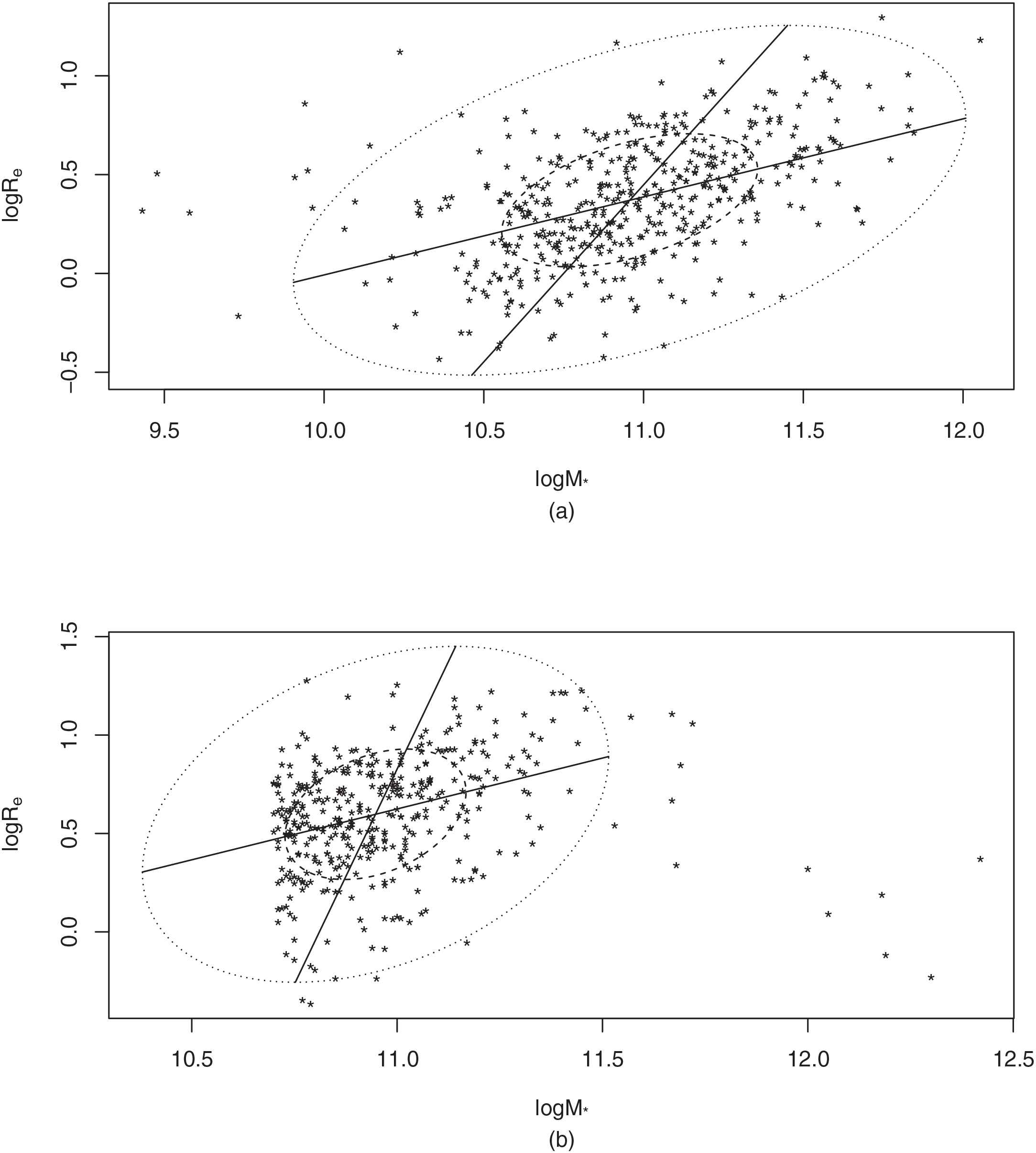
An important area of study in astronomy is the formation and evolution of a certain kind of galaxies called early-type galaxies (ETGs) [1,2]. Here, data are collected from different sources and therefore needed to be checked for compatibility before pooling them together for further study. So, we perform compatibility test between the first data set containing 465 ETGs in the redshift range 0.2<z<2.7, collected from [21], and the second data set consisting 397 ETGs in the redshift range 0<z<2.5, collected from [22], on mass-size parameter space. We draw a bivariate boxplot (Fig. 1) using robust biweight M estimators of correlation, scale, and location [23] (for practical implementation see, [24]) on mass-size observations. Figure 1 shows that both the data sets are affected by outliers, which encourages us to apply our test to these data sets of quite largesizes. The p-value based on HT is 0; and the totals of the p-values for the other tests, with the lower α =0.05 points for B=500, are computed as test,∑i=1n1pi,pα=JK,233.11,229.34,JKa,234.71,231.92 and T~,158.71,149.37. As it is always computationally convincing to take the data set of smaller size as the first data set, we perform the following tests interchanging the data sets and get test, ∑i=1n1pi,pα=JK,74.10,71.87,JKa,70.40,67.16 and T~,6.25,4.39. As HT is supposed to be misleading in such situation, we can ignore it; and the p–values of the other tests support compatibility of the two data sets.

Figure 1

Bivariate boxplot on the mass (logM_*) versus size (logR_e) parameter space for (a) the first data set and (b) the second data set, where the observations lying outside the outer ellipse indicate the potential outliers.

5. CONCLUSION

We propose a nonparametric test using Wilcoxon rank-sum test statistics on distances between observations for each of the components. The test is asymptotically distribution-free under certain conditions. The simulation study shows that the test is unbiased and its power is strictly increasing in the sample sizes and/or in the number of components, provided p<<N, which encourages its applicability to multivariate large sample astronomical data sets. In the presence of outliers or sparsely distributed data where HT fails, the performance of our proposed test, measured in terms of power, is the best among the possible competitors. For distribution i, HT is optimal but under all the models power of T~ becomes very close to 1 for n1=n2=100 with p=10. It guarantees its good performance for the parent distributions like multivariate normal when the sample sizes are large. It is to be noted that in greater effect of outliers as in distribution iii than in distribution ii, T~ performs better than JK, JKa with higher efficacy. It indicates the proposed test's robustness under the presence of unusual observations in the parent distributions. JK and JKa not only get outperformed in the above stated situations but also their powers may become significantly worse for increasing values of p. However, our test being maximized over the components gets only better with increasing p, provided p<<N. Unlike HT, our test is computable for p>N, but not suitable for use, since the test depends on the central limit theorem, which does not hold for large p. As our objective is to provide a test for large sample data with p<<N, we do not concern this problem here, while our future project is to provide tests for large-dimensional data.

ACKNOWLEDGMENTS

The authors would like to thank the editor-in-chief and the anonymous referees for publication of the manuscript in the present form.