
Gaussian Copula–based Regression Models for the Analysis of Mixed Outcomes: An Application on Household's Utilization of Health Services Data
- DOI
- 10.2991/jsta.d.190306.009How to use a DOI?
- Keywords
- Copula models; mixed outcomes; sampling weights; marginal model
- Abstract
In analyzing most correlated outcomes, the popular multivariate Gaussian distribution is very restrictive and therefore dependence modeling using copulas is nowadays very common to take into account the association among mixed outcomes. In this paper, we use Gaussian copula to construct a joint distribution for three mixed discrete and continuous responses. Our approach entails specifying marginal regression models for the outcomes, and combining them via a copula to form a joint model. Closed form for likelihood function is obtained by considering sampling weights. We also obtain the likelihood function for mixed responses where one of the responses, time to event outcome, may have censored values. Some simulation studies are performed to illustrate the performance of the model. Finally, the model is applied on data involving trivariate mixed outcomes on hospitalization of individuals, based on the survey of household's utilization of health services.
- Copyright
- © 2019 The Authors. Published by Atlantis Press SARL.
- Open Access
- This is an open access article distributed under the CC BY-NC 4.0 license (http://creativecommons.org/licenses/by-nc/4.0/).
1. INTRODUCTION
Many statistical applications especially in official statistics involve the collection of multivariate data comprising of a mixture of correlated discrete and continuous responses. Mixed outcomes are ubiquitous in applications and can be also found in health surveys where data may involve a patient choice of healthcare unit, her/his state of health, her/his hospital cost, her/his length of stay in hospital, result of hospitalization, and type of received services along with a number of quantitative demographic and health-related variables. Analyzing each response separately may give misleading results and multivariate modelling of such data often leads to complications in practice due to a relative lack of existence of standard models.
Factorization approach directly specify the joint distribution of variables as the product of a conditional distribution of a set of variables given other variables and a marginal distribution of the others [1].
Indirect approaches to specifying mixed outcomes joint distribution have also been studied. One approach introduces shared or correlated random effects to incorporate correlations between variables in the resulting joint model. The basic idea in this approach is to use random effects to build in correlation between mixed variables [2, 3, 4, 5, 6].
As mentioned, there is so many ways to consider the correlation structure between mixed correlated responses. When mixed responses are recorded on different scales, the copula approach is one of the best to consider the dependence structure. Therefore, a recent alternative strategy involves the use of copulas, as discussed by Sklar [7] who established theoretical basis and by Embrechts et al. [8] who make copulas popular in finance. Copulas incorporate the information on the dependence structure between two or more random variables. A copula is a multivariate probability distribution for which the marginal probability distribution of each variable is uniform and copulas are used to describe the dependence between random variables. If this dependency ignores, it may lead to wrong inference. Some of the literature on copulas focusses on the bivariate case. In this case, the approach relates an arbitrary joint distribution
Different copula models are also used in this situation. Nikoloulopoulos and Karlis [18] used multivariate logit copula and de Leon and Wu [19] used copula-based regression models for a bivariate mixed discrete and continuous outcome [20–23]. Recently, Jiryaie et al. [24] use Gaussian copula distributions for mixed data, with application in discrimination. Also, Stober et al. and Zilko and Kurowicka [25, 26] used copula-based regression models for mixed discrete and continuous outcomes.
A large number of researches have concentrated their attention on the field of reliability and cost–benefit analysis (CBA) with a copula approach [27, 28]. CBA is a systematic approach to estimate the strengths and weaknesses of alternatives. The CBA is also defined as a systematic process for calculating and comparing benefits and costs of a decision, policy, or project. As an example, in our applied data set on hospitalization of individuals, based on the survey of household's utilization of health services (UHS), the benefit of increasing literacy on raising the probability of a full recovery, in relatively short time and low cost, will be illustrated.
In this paper, a closed form for the likelihood, considering three correlated random variables, is given where sampling weights are also taking into account (these weights have not been considered by others). Since applied data set in this paper is from sampling survey, we weigh the data on each member of the sample household to obtain unbiased parameter estimates. This is done in three steps: (1) using base weight which incorporates features of the complex sampling design, multistage sampling, of the UHSs, (2) weighs based on unit nonresponse, and (3) weighs based on population projection. Therefore, the weights should be used in the likelihood and simulation study. These weights somehow increase the number of observations and so more information is incorporated. Consequently, the estimation of standard errors (S.Es.) of parameter estimates would be more precise. We also illustrate the likelihood for three mixed responses where one of the responses, time to event outcome, may have censored values.
The paper is organized as follows. In Section 2, we describe the data set. In Section 3, we introduce a class of copula-based regression models for trivariate mixed outcomes, by considering sampling weights. In this section, we also consider joint modeling of three outcomes, an ordinal outcome (result of hospitalization), a time to event outcome (duration of hospitalization), and a Gaussian continuous outcome (logarithm of cost of hospitalization). Some statistical issues in analyzing mixed outcomes surveys such as sampling weights and censoring are overcame in this section. For each case, the likelihood function is given. In Section 4, some simulation studies are performed for illustration of the performance of the model. In Section 5, data on hospitalization of individuals from survey of household's UHSs are used to illustrate our methodology. Section 6 gives some conclusion.
2. MOTIVATION: HOUSEHOLD'S UTILIZATION OF HEALTH SERVICES DATA
In this section, we will describe the household's UHSs data. The three selected response variables, extracted from these data, are duration and costs of hospitalization as continuous variables and result of hospitalization as a discrete variable. In this section, some factors that affect the behavior of responses will be descriptively examined.
The Iranian 2015 UHS survey was designed and implemented with the aim of identifying the needs of individuals and households to get health services, to be sure of availability of services and to use provided services. Designing of this survey was done regarding to some environmental, economic, social, and political factors impacted on creating health inequalities between different groups of population. The information required for calculating health equity indices and indicators in UHS were gathered through a representative sample selected from different social groups of the population. Many researches are done in different countries based on data on UHS. Garcia-Subirats et al. [29] investigated inequities in access to healthcare in different health systems. Also, Bastos et al. [30] estimate the healthcare utilization and factors influencing it in the public sector in Brazil.
In Iran, this cross-sectional household survey was implemented by Statistical Research and Training Center and the Statistical Centre of Iran (SCI) in cooperation with the Ministry of Health and Medical Education and the National Institute of Health Research. Sample size was 22,470 households and questionnaires were completed with face to face interview with household members. The survey has been implemented in fall of 2014 and all of the information are gathered from respondents in the time of the survey. However, the reference time of some questions such as outpatient and inpatient health services are different. Information about outpatient health service was gathered for the two last weeks before survey and information about the inpatient health service was gathered for a year from 2013 fall to survey time. In the needs and inpatient services section, the survey questionnaire was designed on the needs of individual members of the sample households to hospital (or health facility) during the fall of 2013 until the survey time and in the case of need for hospitalization, name of needs, area of creation (feeling sick or medical guidance), and how to deal with each of them were determined. For individuals who their needs led to stay in hospital (or health facility), evaluation of each inpatient was recorded by household member. For these people, in addition to individual and household information, other information such as the type of hospital, the number of hospitalizations, the waiting period, the works undertaken, the costs of hospitalization, and the result of hospitalization were registered in the questionnaires and gathered at survey time. The results show that the number of households in the sample who have been hospitalized and their data was collected completely in the survey was 2486 households. In this paper, some models were fitted based on the completed sample. The characteristics for selected response variables along with factors that affect the behavior of response variables were also examined. The selected three response variables include duration of hospitalization, costs of hospitalization, and result of hospitalization.
Cost of hospitalization is a continuous variable recorded in rials and the natural logarithm of this variable is used to ensure normality of the response. Duration of hospitalization in days is the second continuous response and the result of hospitalization, as the third response, is an ordinal variable categorized as full recovery, partial recovery, and ineffective admitted. To study the behavior and the factors influencing the response variables, explanatory variables such as residence area, gender, type of hospital, literacy status, activity status, marriage status, and services are extracted from questionnaires of UHS survey and used for the analysis. The descriptive statistics of responses and also the distribution of data in different levels of each explanatory variable are given in Table 1. This table shows that
| Continuous response variables | Level | No. of observation | Mean |
|---|---|---|---|
| log (cost of hospitalization) | - | 2486 | 13.0 |
| Duration of hospitalization | - | 2486 | 3.77 |
| Ordinal response variable | Level | No. of observation | Percentage |
| Result of hospitalization | Full recovery | 1171 | 47.1 |
| Partial recovery | 1119 | 45. | |
| Ineffective admitted | 196 | 7.9 | |
| Covariate variables | Level | No. of observation | Percentage |
| Residence area | Urban | 1669 | 67.1 |
| Rural | 817 | 32.9 | |
| Gender | Male | 1002 | 40.3 |
| Female | 1484 | 59.7 | |
| Type of hospital | Governmental | 1721 | 69.2 |
| Private | 491 | 19.7 | |
| Others | 274 | 11.1 | |
| Literacy status | Illiterate | 707 | 28.4 |
| Diploma | 1452 | 58.4 | |
| Higher education | 327 | 13.2 | |
| Activity status | Employed | 608 | 24.5 |
| Unemployed | 122 | 4.9 | |
| Inactive | 1756 | 70.6 | |
| Marriage status | Married | 2014 | 81.0 |
| Divorced-widow | 234 | 9.4 | |
| Not married | 238 | 9.6 | |
| Services | Specification | 149 | 6.0 |
| Treatment | 43 | 1.7 | |
| Surgery | 691 | 27.8 | |
| Medico | 844 | 34.0 | |
| Rehabilitation | 308 | 12.4 | |
| Child birth | 451 | 18.1 |
Descriptive statistics of responses and covariates.
Figure 1 shows histogram of the natural logarithm of the costs of hospitalization. Figure 2 shows the relationship between different covariates and logarithm of cost of hospitalization by box plots. This figure reveals that the type of hospital and service are important factors on this response. Figure 3 gives stackplots of results of hospitalization versus gender and economic activity status. Based on this figure, the subpopulation of women and men have different patterns of result of hospitalization, that is, among the men subpopulation, partial recovery has the highest percentage, but among the women subpopulation, full recovery has the highest percentage. Also, the subpopulation of employed, unemployed, and inactive people have different patterns of result of hospitalization. Among the unemployed subpopulation, partial recovery has the highest percentage.
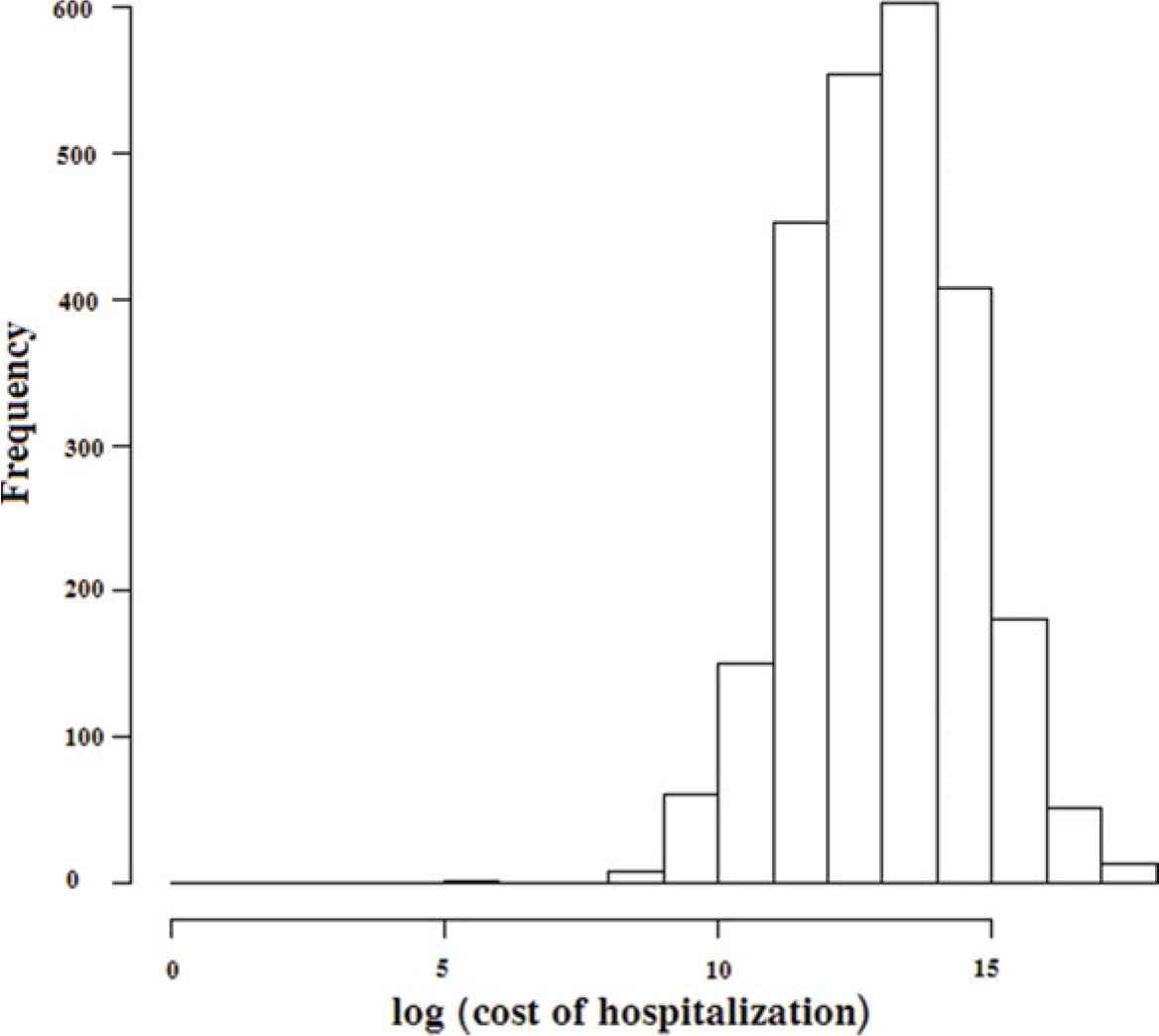
Histogram of natural logarithmic of hospital costs.
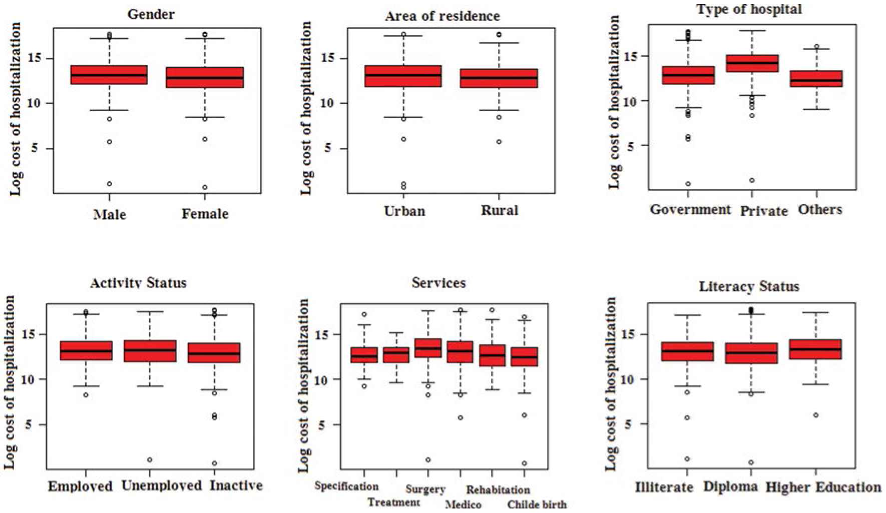
The box plot of logarithm of cost of hospitalization by different covariates.
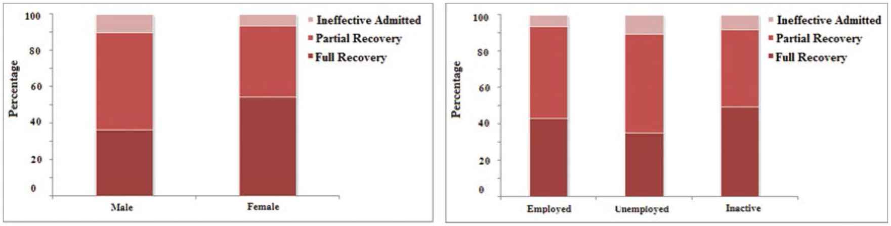
The relative distribution of result of hospitalization by gender and economic activity status.
For a primary description of the explanatory variables on duration of hospitalization, Fig. 4 shows Kaplan–Meier estimators of the survival curves of duration of hospitalization for different covariates groups by considering individual weights. Description of this figure is simple, for example, according to Fig. 4(a) males have longer duration of hospitalization than that of females. Duration of hospitalization in government hospitals is longer than that of private hospitals. Also, people with higher education have smaller duration of hospitalization than that of people who are illiterate or diploma. However, these interpretations are only correct marginally and in the presence of other covariates, using a statistical model, we may find more realistic interpretation. Figure 5 as a survival curve of duration of hospitalization in different combination level of gender and literacy shows that the lowest duration of hospitalization is for female with higher education, but for male, different levels of literacy have nearly the same duration. This means that we need to consider the interaction effect of gender and literacy.
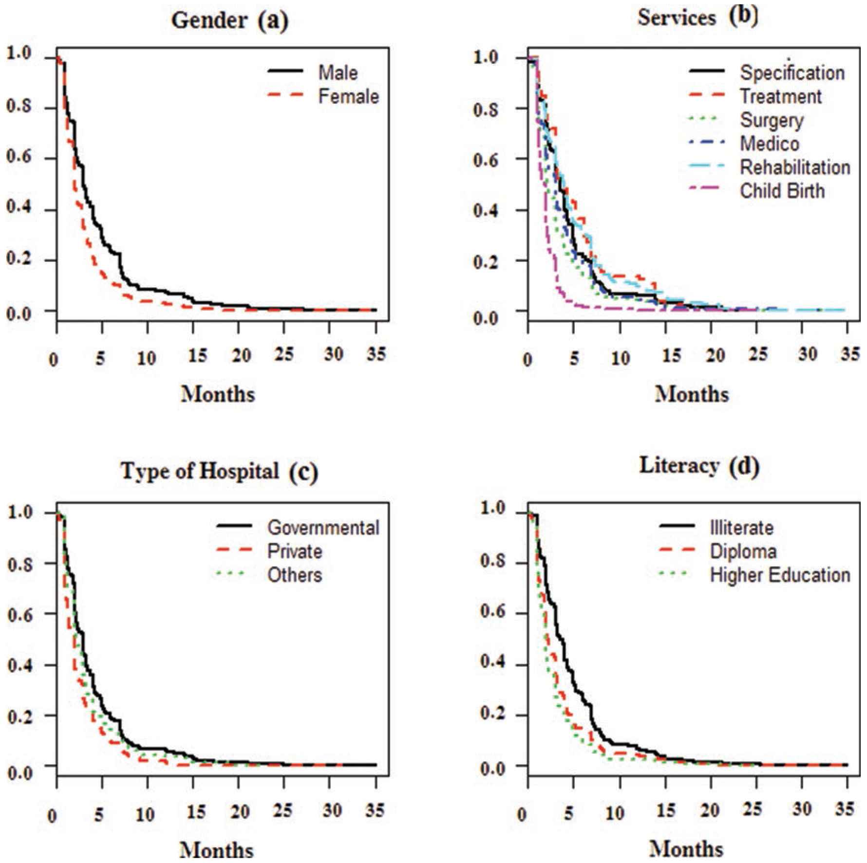
Survival curve of duration of hospitalization on covariates groups, (a) gender, (b) services, (c) type of hospital, (d) literacy.

Survival curve of duration of hospitalization in different combination level of gender and literacy.
3. JOINT MODEL FOR THREE MIXED VARIABLE OUTCOMES
In this section, copula-based regression models for the analysis of three correlated mixed outcomes are discussed. We use Gaussian copula to construct a joint distribution for the three mixed responses. In this approach, we specify marginal regression models for the outcomes, and combine them via a copula to form a joint model. The closed form for likelihood function is also obtained by considering some sampling weights. We also obtain the likelihood function for mixed responses where one of the responses, time to event outcome, may have censored values.
Consider correlated mixed outcomes
Assume
As we have cut points parameters
For continuous variable, we consider
Correlation matrix
Here, the marginal distributions
The joint distribution of
Therefore (vide appendix)
The other joint distribution except
In the same manner, the joint density function of
We also obtain the likelihood function for mixed responses where one of the responses, time to event outcome, may have censored values. In this case,
Let
This likelihood is different with the likelihood given in Eq. (4), as if consider censoring for some outcomes of the time to event.
4. SIMULATION STUDY
In this section, some simulation studies are conducted to illustrate the performance of the proposed model. The structures, that will be used in this section, are considered to be similar to structures we need for analyzing our real data set. In this simulation study, we simulate data from a correlated mixed outcomes including continuous, time to event, and ordinal responses. Also, the effect of varying values of correlation matrix are considered. In another simulation study, the effect of using Gaussian copula on the data generated by non-Gaussian copulas such as Clayton, Frank, Gumbel, and t-copula are also investigated. In this section, two kinds of dependence (Kendall's
Two simulation studies with sample size
Also, a Weibull model is considered for the time to event outcome with the following linear predictor:
As mentioned before, copulas provide a natural way to study and measure dependency between random variables. In order to analyze dependence of multivariate distributions, two important measures of dependence known as Kendall's
For the bivariate Gaussian distribution
In this section, for three random variables Z, Y, and T, the pattern of correlations of pairs
The results of these simulation studies are presented in Table 2. This table contains estimated values of parameters, S.Es.), relative biases (Rel. Bias), and mean square errors (MSEs). These criteria are define as
| N= 200 | N= 1000 | ||||||||
|---|---|---|---|---|---|---|---|---|---|
| Par | Real Value | Est. | S.E. | MSE | Rel. Bias | Est. | S.E. | MSE | Rel. Bias |
| 3 | 3.171 | 0.464 | 0.244 | 0.057 | 3.021 | 0.1725 | 0.030 | 0.007 | |
| 2 | 1.993 | 0.074 | 0.005 | −0.003 | 2.000 | 0.036 | 0.001 | 0.000 | |
| 1 | 1.004 | 0.067 | 0.004 | 0.004 | 0.998 | 0.030 | 0.001 | −0.001 | |
| 3 | 2.997 | 0.121 | 0.015 | −0.001 | 2.998 | 0.055 | 0.003 | −0.000 | |
| 2 | 2.029 | 0.117 | 0.015 | 0.015 | 2.006 | 0.051 | 0.002 | 0.003 | |
| −2 | −2.023 | 0.131 | 0.017 | 0.015 | −2.000 | 0.058 | 0.003 | 0.000 | |
| 2 | 2.024 | 0.113 | 0.013 | 0.012 | 2.003 | 0.050 | 0.002 | 0.002 | |
| 1 | 0.994 | 0.050 | 0.002 | −0.005 | 0.998 | 0.021 | 0.000 | −0.002 | |
| 0.4 | 0.412 | 0.126 | 0.016 | 0.031 | 0.403 | 0.055 | 0.003 | 0.008 | |
| 0.2 | 0.202 | 0.144 | 0.021 | 0.008 | 0.204 | 0.058 | 0.003 | 0.021 | |
| 0.6 | 0.600 | 0.048 | 0.002 | 0.000 | 0.600 | 0.019 | 0.000 | 0.001 | |
| 2 | 2.109 | 0.336 | 0.125 | 0.054 | 2.018 | 0.126 | 0.016 | 0.009 | |
| 1 | 1.049 | 0.233 | 0.057 | 0.049 | 1.003 | 0.090 | 0.008 | 0.003 | |
Est., estimate; MSE, mean of square error; Rel. Bias, relative bias; S.E., standard error.
Results of simulation study, mean (Est.), S.E., Rel. Bias, and MSE of parameter estimate under proposed model with considering covariates using 500 iterations of sample size of 200 and 1000.
In order to investigate the effect of various model misspecifications (under varying values of correlation matrix, or under a non-Gaussian copula) on the results, some other simulation studies are performed. We use other positive define matrices
| Par | Real Value | Est. | S.E. | MSE | Rel. Bias | Est. | S.E. | MSE | Rel. Bias | Est. | S.E. | MSE | Rel. Bias |
|---|---|---|---|---|---|---|---|---|---|---|---|---|---|
| 3 | 3.126 | 0.440 | 0.209 | 0.042 | 3.101 | 0.424 | 0.189 | 0.033 | 3.142 | 0.359 | 0.149 | 0.048 | |
| 2 | 2.000 | 0.088 | 0.008 | 0.000 | 2.000 | 0.079 | 0.006 | 0.000 | 1.993 | 0.085 | 0.007 | −0.003 | |
| 1 | 0.999 | 0.073 | 0.005 | −0.000 | 0.999 | 0.069 | 0.005 | −0.001 | 1.002 | 0.071 | 0.005 | 0.002 | |
| 3 | 2.998 | 0.155 | 0.024 | −0.001 | 2.997 | 0.129 | 0.0166 | −0.001 | 3.006 | 0.129 | 0.016 | 0.002 | |
| 2 | 2.026 | 0.118 | 0.014 | 0.013 | 2.014 | 0.120 | 0.014 | 0.007 | 2.029 | 0.113 | 0.013 | 0.014 | |
| −2 | −2.016 | 0.129 | 0.017 | 0.008 | −2.007 | 0.132 | 0.017 | 0.004 | −2.018 | 0.126 | 0.016 | 0.009 | |
| 2 | 2.021 | 0.111 | 0.013 | 0.010 | 2.014 | 0.114 | 0.0134 | 0.007 | 2.020 | 0.109 | 0.012 | 0.010 | |
| 1 | 0.991 | 0.051 | 0.003 | −0.009 | 0.991 | 0.0511 | 0.003 | −0.009 | 0.989 | 0.048 | 0.002 | −0.011 | |
| 0.098 | 0.147 | 0.022 | −0.021 | 0.412 | 0.121 | 0.015 | 0.030 | 0.709 | 0.074 | 0.005 | 0.013 | ||
| 0.195 | 0.147 | 0.022 | −0.023 | 0.512 | 0.112 | 0.013 | 0.024 | 0.809 | 0.061 | 0.004 | 0.011 | ||
| 0.092 | 0.071 | 0.005 | −0.079 | 0.501 | 0.055 | 0.003 | 0.003 | 0.596 | 0.047 | 0.0022 | −0.005 | ||
| 2 | 2.082 | 0.324 | 0.111 | 0.041 | 2.072 | 0.311 | 0.101 | 0.036 | 2.094 | 0.276 | 0.085 | 0.047 | |
| 1 | 1.041 | 0.227 | 0.053 | 0.041 | 1.026 | 0.226 | 0.052 | 0.026 | 1.045 | 0.2055 | 0.0445 | 0.045 | |
Est., estimate; MSE, mean of square error; Rel. Bias, relative bias; S.E., standard error.
Results of simulation study, mean (Est.), S.E., Rel. Bias, and MSE of parameter estimate under varying values of correlation matrix with components ρ = (ρzy, ρzt, ρyt) using 500 iterations of sample size of 200.
In Table 4, Kendall's
The results of simulation studies under a non-Gaussian copula with using 500 iterations of sample size 200 are also presented in Table 5. Generating data by different copulas [31] such as Clayton, Frank, Gumbel, and t-copula and analyzing them by Gaussian copula show that the generated data by Clayton and T are less sensitive than those of Gumbel and Frank copulas. However, correlation parameters are estimated with some biases using Gaussian copula.
In Table 6, Kendall's
| Real value | |||||||||
|---|---|---|---|---|---|---|---|---|---|
| Par | Est. (S.E.) | Est.(S.E.) | Est.(S.E.) | ||||||
| 0.098 (0.147) | 0.0624 | 0.0936 | 0.412 (0.121) | 0.2703 | 0.3962 | 0.709 (0.074) | 0.5017 | 0.6921 | |
| 0.195 (0.147) | 0.1249 | 0.1865 | 0.512 (0.112) | 0.3422 | 0.4944 | 0.809 (0.061) | 0.5999 | 0.7953 | |
| 0.092 (0.071) | 0.0586 | 0.0878 | 0.501 (0.055) | 0.3340 | 0.4835 | 0.596 (0.047) | 0.4064 | 0.5779 | |
Est., estimate; S.E., standard error.
Kendall's tau (τ) and Spearman's ρ(ρS) values of sample pairs (Z, Y), (Z, T), and (Y, T) calculated under different values of correlation matrix with components ρ= (ρzy, ρzt, ρyt), using 500 iterations of sample size of 200.
| T | Clayton copula | Frank copula | Gumbel copula | ||||||||||||||
|---|---|---|---|---|---|---|---|---|---|---|---|---|---|---|---|---|---|
| Par | Real value | Est. | S.E. | MSE | Rel. Bias | Est. | S.E. | MSE | Rel. Bias | Est. | S.E. | MSE | Rel. Bias | Est. | S.E. | MSE | Rel. Bias |
| 3 | 3.316 | 0.735 | 0.639 | 0.105 | 3.251 | 0.651 | 0.486 | 0.083 | 3.360 | 0.834 | 0.824 | 0.120 | 3.271 | 0.625 | 0.464 | 0.090 | |
| 2 | 2.003 | 0.115 | 0.013 | 0.001 | 1.989 | 0.115 | 0.013 | −0.005 | 1.996 | 0.120 | 0.014 | −0.001 | 2.000 | 0.115 | 0.013 | 0.000 | |
| 1 | 0.994 | 0.100 | 0.010 | −0.006 | 1.002 | 0.100 | 0.010 | 0.002 | 0.997 | 0.110 | 0.012 | −0.003 | 0.999 | 0.092 | 0.008 | −0.000 | |
| 3 | 2.989 | 0.213 | 0.045 | −0.003 | 3.004 | 0.213 | 0.045 | 0.001 | 2.991 | 0.217 | 0.047 | −0.002 | 3.008 | 0.167 | 0.028 | 0.002 | |
| 2 | 2.045 | 0.170 | 0.031 | 0.023 | 2.024 | 0.168 | 0.028 | 0.012 | 2.049 | 0.166 | 0.030 | 0.024 | 2.070 | 0.162 | 0.031 | 0.035 | |
| −2 | −2.033 | 0.196 | 0.039 | 0.016 | −2.021 | 0.200 | 0.040 | 0.010 | −2.054 | 0.201 | 0.043 | 0.027 | −2.062 | 0.186 | 0.038 | 0.031 | |
| 2 | 2.038 | 0.171 | 0.031 | 0.019 | 2.017 | 0.163 | 0.027 | 0.008 | 2.048 | 0.171 | 0.031 | 0.024 | 2.066 | 0.164 | 0.031 | 0.033 | |
| 1 | 0.978 | 0.071 | 0.005 | −0.021 | 0.979 | 0.070 | 0.005 | −0.020 | 0.985 | 0.067 | 0.004 | −0.015 | 0.980 | 0.071 | 0.005 | −0.019 | |
| - | 0.274 | 0.238 | 0.073 | −0.315 | 0.296 | 0.201 | 0.051 | −0.259 | 0.083 | 0.229 | 0.152 | −0.791 | 0.725 | 0.013 | 0.123 | 0.812 | |
| - | 0.088 | 0.248 | 0.074 | −0.558 | 0.295 | 0.203 | 0.050 | 0.475 | 0.064 | 0.228 | 0.071 | −0.679 | 0.722 | 0.125 | 0.288 | 2.609 | |
| - | 0.299 | 0.109 | 0.102 | −0.500 | 0.318 | 0.102 | 0.090 | −0.469 | 0.077 | 0.097 | 0.282 | −0.870 | 0.693 | 0.058 | 0.012 | 0.155 | |
| 2 | 2.199 | 0.538 | 0.328 | 0.099 | 2.144 | 0.479 | 0.249 | 0.072 | 2.228 | 0.613 | 0.427 | 0.114 | 2.169 | 0.441 | 0.222 | 0.084 | |
| 1 | 1.082 | 0.342 | 0.124 | 0.082 | 1.074 | 0.320 | 0.107 | 0.074 | 1.099 | 0.3714 | 0.147 | 0.099 | 1.089 | 0.320 | 0.110 | 0.089 | |
Est., estimate; MSE, mean of square error; Rel. Bias, relative bias; S.E., standard error.
Results of simulation study, mean (Est.), S.E., Rel. Bias, and MSE of parameter estimate under different copula with considering covariates using 500 iterations of sample size of 200.
| T | Clayton copula | Frank copula | Gumbel copula | |||||||||
|---|---|---|---|---|---|---|---|---|---|---|---|---|
| Par | Est. (S.E.) | Est.(S.E.) | Est.(S.E.) | Est. (S.E.) | ||||||||
| 0.274 (0.238) | 0.176 | 0.262 | 0.296 (0.201) | 0.191 | 0.284 | 0.083 (0.229) | 0.053 | 0.079 | 0.725 (0.013) | 0.516 | 0.708 | |
| 0.195 (0.088) | 0.056 | 0.084 | 0.512 (0.295) | 0.190 | 0.283 | 0.064 (0.228) | 0.041 | 0.061 | 0.722 (0.125) | 0.513 | 0.705 | |
| 0.092 (0.299) | 0.193 | 0.286 | 0.501 (0.318) | 0.206 | 0.305 | 0.077 (0.097) | 0.049 | 0.073 | 0.693 (0.058) | 0.487 | 0.675 | |
Est., estimate; S.E., standard error.
Kendall's tau (τ) and Spearman's ρ(ρS) values of sample pairs (Z, Y), (Z, T), and (Y, T) calculated under different copula with considering covariates using 500 iterations of sample size of 200.
5. APPLICATION TO THE HOUSEHOLD'S UHS DATA
In this section, we use the household's UHS data implemented by SCI in 2015 to illustrate our methodology. Three interested variables, length of stay in hospital, hospital costs, and results of hospitalization are considered as correlated mixed variables. The data involve N =2486 patients of different ages who are hospitalized. The interest lies in simultaneously linking three outcomes, namely, logarithm of hospital costs,
We assume
The results of using Model I show that as age increases, the probability of having ineffective admitted increases. Males are more likely to fully or partially recovered than females. Employed people are more likely to fully or partially recovered than inactive and unemployed people. People with service of child birth are more likely to fully or partially recovered than other people. The results of using Model I show that the cost of hospitalization for older people is more than that of younger people. Also, the cost of hospitalization in private and government hospitals are more than those of other hospitals. The costs of hospitalization in private hospitals are more than that of government hospitals. Cost of hospitalization in rural area is less than that of urban area. Also, the cost of hospitalization of employed and unemployed people is more than that of inactive people. This cost for employed people are more than that of unemployed people.
Males have longer duration of hospitalization than that of females. Duration of hospitalization in government hospitals is shorter than that of other hospitals. But, duration of hospitalization in private hospitals is longer than that of other hospitals. Also people who are illiterate or diploma have shorter duration of hospitalization than that of people with higher education. People who received medico, rehabilitation, specification, treatment, or surgery services, have shorter duration of hospitalization than those of people who received child birth services. The results of Table 7 show that three response variables are significantly correlated. Also, the Kendall's
In order to compare the different models, the AIC is computed for joint and separate models in Table 7. Given any two or more estimated models, the model with the lowest value of AIC is the one to be preferred. The results of Table 7 shows that Model I (joint model), has a better fit of the data.
| Model I | Model II | |||
|---|---|---|---|---|
| Par (X) | Est. | S.E. | Est. | S.E. |
| 0.0076 | 0.0000 | 0.0080 | 0.0000 | |
| −0.0810 | 0.0019 | −0.0862 | 0.0019 | |
| Economic activity status (Baseline: Inactive) | - | - | - | - |
| −0.2237 | 0.0021 | −0.2282 | 0.0021 | |
| 0.0068 | 0.0035 | 0.0242 | 0.0035 | |
| Services (Baseline: Child birth) | - | - | - | - |
| 1.9135 | 0.0040 | 1.8956 | 0.0040 | |
| 2.0966 | 0.0040 | 2.0788 | 0.0040 | |
| 2.4878 | 0.0043 | 2.4712 | 0.0043 | |
| 2.0362 | 0.0045 | 2.0363 | 0.0045 | |
| 1.6644 | 0.0013 | 1.6668 | 0.0013 | |
| 12.1225 | 0.0042 | 12.0664 | 0.0042 | |
| 0.0045 | 0.0000 | 0.0061 | 0.0000 | |
| Type of hospital (Baseline: Others) | - | - | - | - |
| 0.3532 | 0.0028 | 0.3607 | 0.0028 | |
| 1.6464 | 0.0033 | 1.6464 | 0.0033 | |
| Residence area (Baseline: Urban) | - | - | - | - |
| −0.1873 | 0.0019 | −0.1358 | 0.0020 | |
| Economic activity status (Baseline: Inactive) | - | - | - | - |
| 0.2311 | 0.0021 | 0.2169 | 0.0022 | |
| 0.1536 | 0.0040 | 0.2134 | 0.0042 | |
| Services (Baseline: Child birth) | - | - | - | - |
| 0.5095 | 0.0029 | 0.4138 | 0.0029 | |
| 0.4180 | 0.0029 | 0.3240 | 0.0029 | |
| 0.2690 | 0.0035 | 0.1769 | 0.0035 | |
| 1.4545 | 0.0006 | 1.4456 | 0.0006 | |
| −1.3045 | 0.0034 | −1.3447 | 0.0035 | |
| Gender (Baseline: Female) | - | - | - | - |
| 0.4810 | 0.003 | 0.5068 | 0.0034 | |
| Type of hospital (Baseline: Others) | - | - | - | - |
| −0.1034 | 0.0020 | −0.1139 | 0.0020 | |
| 0.3022 | 0.0023 | 0.3011 | 0.0023 | |
| Literacy status (Baseline: Higher education) | - | - | - | - |
| −0.3311 | 0.0031 | −0.3199 | 0.0032 | |
| −0.0940 | 0.0026 | −0.0905 | 0.0027 | |
| Literacy status*Gender(Baseline: Higher education*Male) | - | - | - | - |
| −0.2711 | 0.0041 | −0.4928 | 0.0020 | |
| −0.1002 | 0.0035 | −0.5762 | 0.0020 | |
| Services (Baseline: Child birth) | - | - | - | - |
| −0.5158 | 0.0020 | −0.8803 | 0.0025 | |
| −0.6033 | 0.0020 | −0.2938 | 0.0042 | |
| −0.8984 | 0.0024 | −0.0758 | 0.0037 | |
| 1.3052 | 0.0005 | 1.3073 | 0.0005 | |
| Correlation Structure | ||||
| 0.1441 | 0.0007 | - | - | |
| 0.1181 | 0.0008 | - | - | |
| 0.2826 | 0.0006 | - | - | |
| AIC | 24,356,940 | 24,585,384 | ||
| BIC | 24,357,144 | 24,585,570 | ||
| HQC | 24,356,874 | 24,585,324 | ||
AIC, Akaike Information Criterion; Est., estimate; S.E., standard error.
Parameter Est. and S.Es. obtained by Gaussian copula to construct a joint distribution for three discrete and continuous responses in household's utilization of health services data (Model I: joint model with some interactions effects, Model II: separate models with some interaction effects).
The predictive plot of survival curve of duration of hospitalization in different combination levels of gender and literacy in Fig. 6, obtained by the results of fitted Model I, shows the same pattern as that of Fig. 5 which emphasizes the well performance of the model. In this plot, the values of other covariates are prefixed. We consider gender as a male, type of hospital as a governmental, and services as rehabilitation.
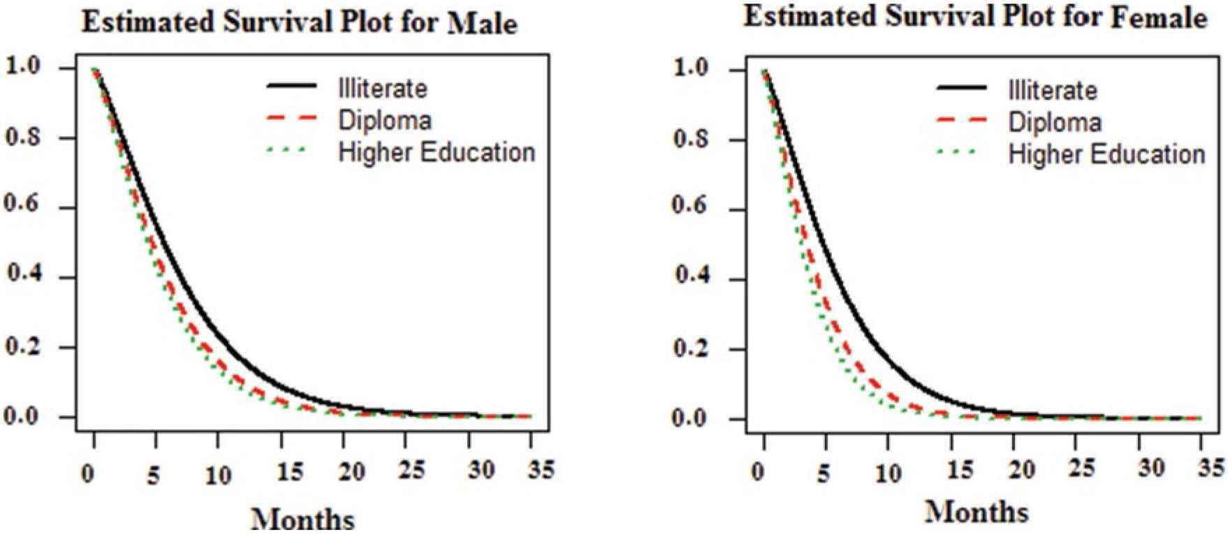
Predictive plot of survival curve of duration of hospitalization in different combination levels of gender and literacy.
In order to estimate the benefit of increasing literacy, in terms of raising the probability of a full recovery in relatively short time of stay in hospital and low cost of the hospitalizations, the conditional probability of full recovery given short time of stay in hospital and low cost of the hospitalizations should be determined for different levels of literacy. By last line of Eq. (8) and
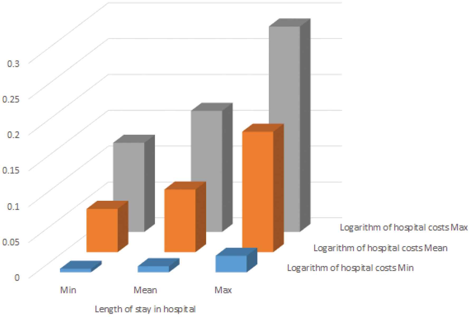
Probability of a full recovery given different combination levels of length of stay in hospital and cost of the hospitalizations.
The probability of a full recovery in different combination levels of length of stay in hospital (minimum, mean and maximum) and cost of the hospitalizations (minimum, mean, and maximum) in Fig. 7, obtained by the results of fitted Model I, shows that by increasing the length of stay in hospital and cost of the hospitalizations, the probability of a full recovery will be increased. Analyzing the residuals for the continuous variable of cost shows that the response 42 is an outlier, but removing this individual and analyzing the remaining data does not affect our results.
6. CONCLUSION
In this paper, copula-based regression models for mixed discrete and continuous outcomes, with application in household's UHS data were discussed. Proposed model was also illustrated on some simulated data. It was shown how to construct a joint model for three discrete and continuous responses using Gaussian copula. Likelihood of this model is able to consider the important information of sampling weights. In addition to having continuous and ordinal responses, we may have a recorded nominal response. This paper can be extended to consider cases including a nominal response. For nominal responses, another latent variable should be defined [33].
7. APPENDIX
In this appendix we find the joint trivariate distribution,
References
Cite this article
TY  - JOUR
AU  - Z. Rezaei Ghahroodi
AU  - R. Aliakbari Saba
AU  - T. Baghfalaki
PY  - 2019
DA  - 2019/07/11
TI  - Gaussian Copula–based Regression Models for the Analysis of Mixed Outcomes: An Application on Household's Utilization of Health Services Data
JO  - Journal of Statistical Theory and Applications
SP  - 182
EP  - 197
VL  - 18
IS  - 3
SN  - 2214-1766
UR  - https://doi.org/10.2991/jsta.d.190306.009
DO  - 10.2991/jsta.d.190306.009
ID  - Ghahroodi2019
ER  -