Journal of Statistical Theory and Applications

Volume 18, Issue 3, September 2019, Pages 323 - 328

On the Asymptotic Behavior in Random Fields: The Central Limit Theorem

Authors
Mohammad Mehdi Saber1, Zohreh Shishebor2, *, Behnam Amiri2
1Department of Statistics, Higher Education Center of Eghlid, Eghlid, Iran
2Department of Statistics, Shiraz University, Shiraz, Iran
*Corresponding author. Email: shisheb@shirazu.ac.ir
Corresponding Author
Zohreh Shishebor
Received 1 October 2017, Revised 1 April 2018, Accepted 1 May 2018, Available Online 19 September 2019.
DOI
10.2991/jsta.d.190830.001How to use a DOI?
Keywords
Central Limit Theorem; Increasing domain sampling; m-dependent
Abstract

The aim of this paper is to provide an applicable version of Central Limit Theorem for strictly stationary m-dependent random fields on a lattice. The type of sampling is considered increasing domain sampling.

Copyright
© 2019 The Authors. Published by Atlantis Press SARL.
Open Access
This is an open access article distributed under the CC BY-NC 4.0 license (http://creativecommons.org/licenses/by-nc/4.0/).

1. INTRODUCTION

A random field (RF), Z=Zs,s∈S, S⊆Rk, is a collection of random variables indexed by s. RFs are used in a variety of fields including geology, geography, biology, earth science, health, medicine, image processing, etc. A lot of research has been done in this field during the past few years; nonetheless many key statistical topics have not been answered yet. The aim of this study is to investigate the asymptotic properties of some statistics in RFs under increasing domain sampling. Two important statistics are the sample mean and sample variance, which are used to estimate the mean and variance of a population, respectively. Usually the exact distributions of these two statistics is unknown. In this study, we are interested in asymptotic behavior of sample mean Z¯n and its limiting distribution. So, different versions of spatial sampling are needed to be explained. “When the sampling region remains bounded as n tends to infinity but the sample size n grows to infinity it is called infill domains sampling” [1]. Lahiri [2] proved that in this case, the Central Limit Theorem (CLT) for ∑i=1nZi cannot be hold. “If sampling region becomes unbounded with n and the structure of Sn is such that there is a minimum distance between any two sites for all n, it is called increasing domain sampling” [1] which is our focus in this work. “The third one is mixed (or nearly infill) domain sampling, where the infill domain sampling is mixed with the increasing domain sampling.” Lahiri [3] established a spatial CLT for the nearly infill domain sampling. He considered both fixed and random designs. Following the work of Lahiri, Byeong U. Park et al. [4] earned a CLT for m-dependent and stationary RFs with more convenient conditions satisfied.

Various types of CLT for spatial processes have been considered by some authors. Among them, Stein [5] proved consistency and CLT for weighted sum of RFs under stochastic sampling. Jenish and Prucha [6] proved CLTs and uniform law of large numbers for arrays of RFs. They [7] also, proved a CLT and law of large numbers under near-epoch dependence. A Lindeberg CLT for strictly stationary RFs was provided by Cristina Tone in 2013 [8]. Maltz and Samur [9] worked on a uniform CLT on rectangles for functions of mixing RFs. Berkes et al. [10] have achieved some asymptotic results for the empirical process of stationary sequences. Machkouri et al. [11] have proved a CLT for stationary and m-dependent RFs. In this work a CLT for strictly stationary m-dependent RFs is provided under increasing domain sampling. The interesting finding in our study is that the proposed theorem only needs to have finite variance.

The paper is organized as follows. In Section 2, some requirements for CLT such as, the asymptotic behavior of ∑i=1nZinα for some appropriate values of α for two cases of m-dependency and ergodicity are studied. Section 3 will give the limiting distribution of Z¯n in the case that Z is a strictly stationary m-dependent RF (Theorem 2). A conclusion is given in Section 4.

2. BASIC CONCEPTS AND PRELIMINARY RESULTS

Here and after we suppose that the type of sampling is increasing domain sampling. In linear algebra, the size of a vector x is named the norm of x. There are different kinds of norms on Rk. In order to have less complicated computations the max norm is applied here which is defined as follows:

‖x‖∞=max|x1|,…,|xk|forx=(x1,…,xk)∈Rk.

We define two types of sets

Bx0,r=x∈Rk| ‖x−x0‖∞≤r               closed Ball,

Sx0,r=x∈Rk| ‖x−x0‖∞=r                  sphere.

In the two cases, r is called the radius and x0 is the center. For clarification, we emphasize that Bx0,r is a solid square and Sx0,r is a square. Also, it is worth to mention that max and Euclidian norms are equivalent and induce the same topology on Rk. So, all results are valid with the usual Euclidian topology.

Let us define the concepts of stationarity, strict stationarity and m-dependence.

Definition 2.1.

The RF Z=Zs,s∈S⊆Rk is said to be stationary if ∀s,t∈S

(i) EZs=a, (ii) E|Zs|2<∞ and (iii) covZs,Zt=γ‖s−t‖∞

Definition 2.2.

The RF Z=Zs,s∈S⊆Rk is said to be strictly stationary if Zs1+h,…,Zsm+h=D Zs1,…,Zsm, for all s1 , s2,…, sm, h∈S, where D stands for identically distributed.

Definition 2.3.

The RF Z=Zs,s∈S⊆Rk is said to be m-dependent if Zs and Zt are independent for every s,t∈S such that ‖s−t‖∞>m.

Whenever we have weak stationarity, two symbols σ02=varZs and σ‖s−t‖∞2=covZs,Zt are used. For simplicity of notation we write Zi instead of Zsi, when no confusion can arise.

The following result is used to prove the main issue. It also has some direct result concerning the limiting distribution of Zn¯. So we state it as a theorem.

Theorem 1.

Suppose that Λ is an Nk lattice in Rk with coordinates s1,…,sn and cell width δ=1 where n=Nk. Let Z be a mean zero RF on Λ such that VarZi≤c<∞ for all i=1,…,n.

  1. If ρZi,Zj→0, as ‖si−sj‖∞ tends to infinity and if α≥1, then ∑i=1nZinα→L20.

  2. If Z is an m-dependent RF, then ∑S∈AZsnα→L20 for all α>Ln#A2 Lnn, where #A shows the number of members in set A.

  3. If Z is a stationary m-dependent RF, then limn→+∞var∑i=1nZin=σ02+∑j=1m2j+1k−2j−1kσj2.

Proof.

(i) Since ∑i=1nZinα is an unbiased estimator of zero, it is enough to show that Var∑i=1nZinα goes to zero as n goes to infinity. So, let us compute the variance of ∑i=1nZinα.

Var∑i=1nZinα=1n2α∑i=1n∑j=1ncovZi,Zj=1n2α∑i=1n∑j=1nVarZiVarZjρZi,Zj≤cn2α∑i=1n∑j=1nρZi,Zj.

The uniform convergence to zero of the sequence ρZi,Zj, implies that for all ε>0, there exists an integer Nε large enough such that ρZi,Zj≤ε for all Zi and Zj whenever ‖si−sj‖∞>Nε. The number of points in Bsi,Nε are at most 2Nεk. Thus the total number of points with condition ‖si−sj‖∞≤Nε i,j=1,…,n, are at last n2Nεk. The computation of the later inequality can be followed as

cn2α∑i=1n∑j=1nρZi,Zj=cn2α∑i=1n∑j=1nρZi,ZjI‖si−sj‖∞≤Nε  +cn2α∑i=1n∑j=1nρZi,ZjI‖si−sj‖∞>Nε ≤cn2αn2Nεk+n2−n2Nεkε =c1n2α−12Nεk+1n2α−2−1n2α−12Nεkε.

The last term tends to zero as n tends to infinity if α≥1, and this completes the proof of part (i).

(ii) Following the same method as in part (i), we have

Var∑s∈AZsnα≤cn2α∑s∈A∑t∈A|ρZs,Zt| ≤c #A2m+1kn2α.

Let #A∝nq, then if 2α>q results in Var∑s∈AZsnα tends to 0 as n tends to infinity. Note that #A∝nq is equivalent to q∝Ln#ALnn. This completes the proof.

(iii) By m-dependence and stationarity we have

var∑i=1nZi=∑i=1n∑j=1ncovZi,Zj=∑i=1n∑s∈Bsi,mσ‖si−s‖∞2 =∑i∈Q ∑s∈Bsi,mσ‖si−s‖∞2+∑i∉Q ∑s∈Bsi,mσ‖si−s‖∞2.
where Q is the set of all indexes for which #Bsi,m=2m+1k. It is easy to see that #Q=n1k−2mk.

Let us compute the value of the first term in the above expression. By stationarity ∑i∈Q∑s∈Bsi,mσ‖si−s‖∞2= n1k−2mk ∑s∈Bsi,mσ‖si−s‖∞2. The set Bsi,m will be partitioned into m+1 disjoint sets Ssi,j, j=0,…,m. Since for all s∈Ssi,j we have ‖si−s‖∞=j, the value of #Ssi,j must be computed. Clearly Ssi,0=si and #Ssi,0=1. Also, by construction we have #Ssi,j=#Bsi,j−#Bsi,j−1=2j+1k−2j−1k, j=1,…,m.

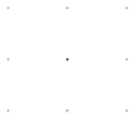
To see more clearly see Fig. 1 for k=2 and j=1. Spurred by this finding we have ∑s∈Bsi,mσ‖si−s‖∞2=σ02 + ∑j=1m2j+1k−2j−1kσj2. To calculate the second term note that |∑s∈Bsi,mσ‖si−s‖∞2|≤|σ02|+∑j=1m2j+1k−2j−1k|σj|2=M<+∞ for i∉Q. Thus, ∑i∉Q∑s∈Bsi,mσ‖si−s‖∞2≤n−n1k−2mkM. Since n−n1k−2mk≤nk−1k∑j=0k−1kj2mk−j, we have ∑i∉Q∑s∈Bsi,mσ‖si−s‖∞2≤nk−1k∑j=0k−1kj2mk−jM. Finally limn→+∞n1k−2mkn=1 and limn→+∞nk−1k∑j=0k−1kj2mk−j Mn=0 which complete the proof.

Figure 1

There are (2(1)+1)2−1=8 points whose distance with bold point is 1.

We finish this section with a direct result of Theorem 1.

Corollary 1.

(Consistency of Z¯n) If Z is a RF with non-zero mean Z¯n→Pμ.

Remark 1.

We point out that the obtained results are maintained under the Euclidian topology, with #Bsi,r≤2r+1k.

3. CLT FOR RFS ON A REGULAR LATTICE

In this section a CLT for strictly stationary m-dependent RFs on a regular lattice under increasing domain sampling has been established. First, let us state the basic lemma from Ferguson ([12], p. 77) in advanced probability.

Lemma 1.

Suppose Yn=Znq+Xnq for n=1,2,… and =1,2,…. If

  1. Xnq→p0 uniformly in n as q tends to infinity,

  2. Znq→DZq, as n tends to infinity for all q,

  3. Zq→DZ, as q tends to infinity,

then, Yn→DZ as n tends to infinity.

Now, we state the CLT and we will prove it using Lemma 1.

Theorem 2.

Let Λ be a square lattice in Rk with coordinates, s1,…,sn and cell width δ=1. Let Z be a strictly stationary m-dependent RF with finite variance σ02 on this lattice. If Tn=∑i=1nZsi, then Tn−n μnσ→DN0,1 where σ 2=σ02+∑j=1m2j+1k−2j−1kσj2 and σ‖si−sj‖∞2=covZsi,Zsj.

Proof.

Without loss of generality we can assume that μ=0. The method of the proof involves splitting the sum Tn into two parts, one being a sum of independent random variables for which the CLT can be applied, and the other sum containing negligible terms. Let n=bm+q+ek, 0≤e<m+q and q>m where m, q and e are positive integers. It is worth to mention that, m,q and e do not depend on n but b increases as n increases. We break the lattice Λ into bk sections Wnu1,…,uk, ui=1,…,b of size m+qk and a remainder Rn. By construction, Rn can be divided into sections that at least one of their dimensions is equal with e. The set Tn can be decomposed as

Tn=∑u1=1b…∑uk=1b∑s∈Wn(u1,…,uk)z(s)+∑s∈Rnz(s).

The section Wnu1,…,uk is broken down into 2k subsections Vt1,t2,…,tku1,…,uk, ti=1,2.

Wnu1,…,uk=∪t1=12…∪tk=12Vt1,t2,…,tku1,…,uk.

The ith dimension of Vt1,t2,…,tku1,…,uk in (2) is equal with q and m for ti=1 and ti=2, respectively. Let Tt1,t2,…,tk=∪u1=1b…∪uk=1bVt1,t2,…,tku1,…,uk. Therefore (1) can be rewritten as

Tn=∑t1=12…∑tk=12∑s∈Tt1,t2,…,tkZs+∑s∈RnZs.

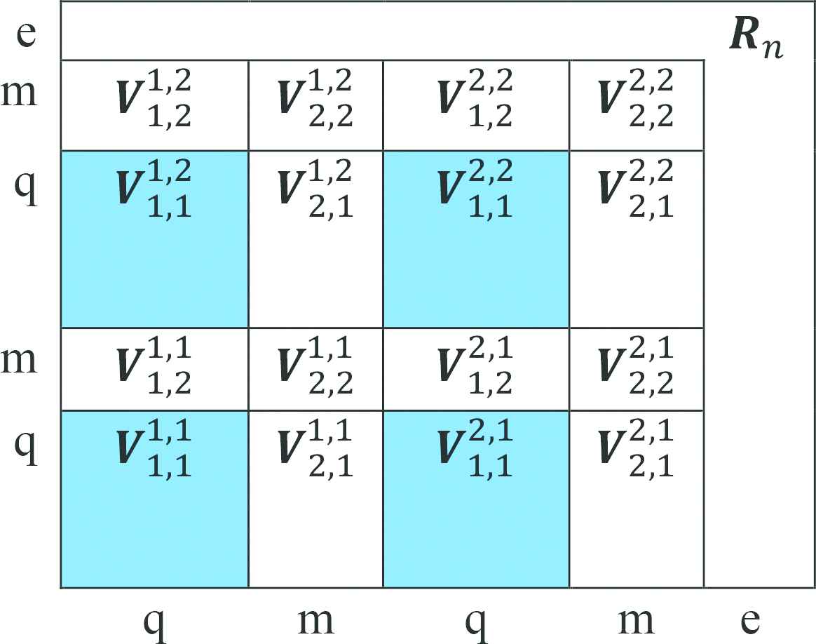
To have a better understanding of definitions see Fig. 2 for the special case k=2 and b=2. To complete the proof, it suffice to apply Lemma 1 for Yn=Tnn, Znq=∑s∈T1,1,…,1Zs+∑s∈RnZsn and Xnq=1n ∑t1=12…∑tk=12∑s∈Tt1,t2,…,tkZst1,…,tk≠1,…,1.

Figure 2

For parameters b=2 and k=2, the lattice has been broken. Here, blue color shows T1,1.

The CLT along with the strict stationarity assumption guarantees that for any fixed q, ∑s∈T1,1,…,1Zsbk→DN0,var∑s∈V1,…,11,…,1Zs. Since limn→∞bkn=1m+qk, it follows from Slutsky theorem that

∑s∈T1,1,…,1Zsn→DN0,var∑s∈V1,…,11,…,1Zsm+qk.

Let rn indicate the number of indices used in Rn. Then,

limn→∞rn k2k−1n=limb→∞kbm+qk−1 ek2k−1bm+q+ek2=kek2k−1.

The first equality comes from the fact that  rn=bm+q+ek−bm+qk and n=bm+q+ek. Since k2k−1>12 for every k, from Part (ii) of Theorem 1, we have that

∑s∈RnZsrn k2k−1→L20 as n→∞.

(5) and (6) imply that

∑s∈RnZsn→L20 as n→∞.

Now it follows from (4) and (7) that Znq→DZq~N0,var∑s∈V1,…,11,…,1Zsm+qk. Finally part (iii) of Theorem 1 implies that Zq→N0,σ2 as q tends to infinity.

It remains to check the first condition of Lemma 1. In part (ii) of Theorem 1 let A be the set Tt1,t2,…,tk, t1,…,tk≠1,…,1 and α=12. Since #A∝qk−1 and n∝qk, we have ∑s∈Tt1,t2,…,tkZsn→P0 as q tends to infinity if 12>Lnqk−12 Lnqk=k−12 k. Clearly the last condition is satisfied for every k. This means that Xnq→P0. as q tends to infinity, uniformly in n.

Wn1,1=V1,11,1+V2,11,1+V1,21,1+V2,21,1, Wn1,2=V1,11,2+V2,11,2+V1,21,2+V2,21,2Wn2,1=V1,12,1+V2,12,1+V1,22,1+V2,22,1, Wn2,2=V1,12,2+V2,12,2+V1,22,2+V2,22,2T1,1=V1,11,1+V1,11,2+V1,12,1+V1,12,2, T1,2=V1,21,1+V1,21,2+V1,22,1+V1,22,2T2,1=V2,11,1+V2,11,2+V2,12,1+V2,12,2, T2,2=V2,21,1+V2,21,2+V2,22,1+V2,22,2

4. CONCLUSION

In this work under increasing domain sampling the asymptotic behavior of ∑i=1nZinα for some appropriate value of α has been given in two cases, the case of ergodicity and the case of m-dependency. In the latter case a version of CLT was given. Extending this work to other sampling modes is an interesting work which it should be stated in the future.

Journal
Journal of Statistical Theory and Applications
Volume-Issue
18 - 3
Pages
323 - 328
Publication Date
2019/09/19
ISSN (Online)
2214-1766
ISSN (Print)
1538-7887
DOI
10.2991/jsta.d.190830.001How to use a DOI?
Copyright
© 2019 The Authors. Published by Atlantis Press SARL.
Open Access
This is an open access article distributed under the CC BY-NC 4.0 license (http://creativecommons.org/licenses/by-nc/4.0/).

Cite this article

TY  - JOUR
AU  - Mohammad Mehdi Saber
AU  - Zohreh Shishebor
AU  - Behnam Amiri
PY  - 2019
DA  - 2019/09/19
TI  - On the Asymptotic Behavior in Random Fields: The Central Limit Theorem
JO  - Journal of Statistical Theory and Applications
SP  - 323
EP  - 328
VL  - 18
IS  - 3
SN  - 2214-1766
UR  - https://doi.org/10.2991/jsta.d.190830.001
DO  - 10.2991/jsta.d.190830.001
ID  - Saber2019
ER  -