In this paper, we consider a numerical pricing of European call and put options under the Heston-Cox-Ingersoll-Ross (HCIR) model. Based on this model, the prices of options are derived by solving a three-dimensional partial differential equation. We generalize a componentwise splitting scheme for solving this equation. The idea of this scheme is to decompose the discretized HCIR partial differential equation into six one-dimensional equations in six fractional time steps. These equations are represented in tridiagonal systems, which are solved by the Thomas algorithm. Moreover, the numerical experiments show that the European option prices are affected by changes in volatility, interest rate, strike price, and correlation factors. Furthermore, numerical experiments compare the calculated prices based on our scheme with the prices reported in the literature.
The Black-Scholes model [1] has been widely used for option pricing. The volatility and the interest rates are both assumed constant in this model. Many studies have shown that better experimental results are obtained when the volatility follows a stochastic process. Therefore, a number of stochastic volatility models have been suggested, including Ball and Roma [2], Fouque et al. [3], Heston [4], Hull and White [5], Schöbel and Zhu [6], Stein and Stein [7]. On the other hand, for the pricing of long-maturity options, adoption of a constant interest rate is contrary to the market reality, see Bakshi et al. [8]. Hence, in some studies, in addition to the volatility, interest rate is modeled by a stochastic process, “as in Refs. [9–12]”. In the literature several suggestions to model the stochastic interest rate are given, including Cox-Ingersoll-Ross [13], Hull-White [14], Vasicek [15].
The model we will consider here is a combination of the famous Heston model [4] for the stochastic volatility and the Cox-Ingersoll-Ross model [13] for the stochastic interest rate, which is called the Heston-Cox-Ingersoll-Ross (HCIR) model. In general, there is no exact solution in the literature for the HCIR model. Grzelak and Oosterlee [16] have presented two projection techniques to drive affine approximations of the HCIR model. Haentjens [17] has presented the numerical solution of HCIR model by alternating direction implicit finite difference (FD) schemes.
The main purpose of this paper is to introduced a numerical method for solving HCIR model. Yanko [18] introduced a componentwise splitting scheme for three-dimensional heat conduction equation with mixed derivatives. Here, we generalize this scheme for decomposition of three-dimensional HCIR partial differential equation. Using this scheme, the HCIR partial differential equation is approximated by solving six tridiagonal systems in six fractional time steps. These tridiagonal systems can be solved using the Thomas algorithm.
This paper is organized as follows. In Section 2 we derive the HCIR PDE for pricing European options, and the associated boundary conditions. In Section 3 we describe a FD discretization of the HCIR PDE. In Section 4 we present a numerical method, based on generalization of componentwise splitting scheme, to solve the PDE to obtain approximations to the prices of the European options. Numerical results are presented in Section 5. The paper ends with conclusions in Section 6.
2. DERIVATION OF THE HCIR PDE
The HCIR model proposed by the Grzelak and Oosterlee [16]. In the HCIR model, both parameters of volatility and interest rate are stochastic. Such that, the volatility process follows the Heston model [4] and the interest rate process follows the Cox-Ingersoll-Ross model [13]. Therefore, the dynamics of underlying asset price st, stochastic volatility νt, and stochastic interest rate rt are given by a system of three stochastic differential equations (SDEs) as follows:
for 0⩽t⩽T with T>0 the given maturity time of the option. Hear, κ and λ determine the mean reversion speed of νt and rt, respectively, η represents the volatility of νt-process, and γ represents the volatility of rt-process, ν¯ and r¯ are the long-run means of νt-and rt-process, respectively. Moreover in Eq. (1), Wts, Wtν, and Wtr are the standard Wiener process, with the correlation structure here given by dWtsdWtν=ρs,νdt, dWtsdWtr=ρs,rdt, and dWtνdWtr=ρν,rdt. The Feller condition for the volatility process is κν¯η2>12, which causes νt to remain strictly positive. The Feller condition for interest rate is λr¯γ2>12, which causes rt to remain strictly positive. In practice, the Feller condition is difficult to satisfy, see [16] for details.
Assume that u(s,ν,r,t) represents the value of a European option at time t. Then, the final condition is given by
where K is the strike price. Hence, the price of a claim on st paying H(s,T) at maturity given by
u(st,νt,rt,t)=Es,ν,r,tH(s,T)e−∫tTr(s)ds.
Note that, the term e−∫tTr(s)ds is the money-saving account which can not be pulled out of the expectation, because interest rate rt is not constant. Hence, we use an auxiliary process of the form dy=−r(t)dt, see, for example, [19]. Therefore, we have
u(st,νt,t,t)=e−yV(st,νt,rt,t),
where, V(st,νt,rt,t)=Est,νt,rt,t(H(s,T)ey(T)) and to the function V(st,νt,rt,t) the Feynman-Kac theorem can be applied. Then, transforming the V(st,νt,rt,t) back to u(st,νt,rt,t) gives the corresponding HCIR PDE which defines the value of a European option as follows:
Before we express the FD approximations for the space variables, we truncate the unbounded domain into a finite computational domain (s,ν,r,τ)∈[0,smax]×[0,νmax]×[0,rmax]×[0,T]. The boundary conditions for the European call option under HCIR model are described in [17], for example. The boundary conditions are
and for the boundary condition at ν=0, we consider inserting ν=0 into the HCIR PDE. This boundary condition has been investigated by Ekström and Tysk [20]. Therefore, the HCIR PDE on the boundary ν=0 reduces to
Finally, the special boundary condition r = 0 is considered similar as the boundary condition at ν=0. Hence, the boundary condition at r = 0, by inserting r = 0 into HCIR PDE, leads to the omission of a number of derivative terms of HCIR PDE:
A European put option with strike price K and maturity time T satisfies the HCIR PDE subject to the following boundary conditions:
u(0,ν,r,τ)=Ke−rτ,(5)
∂u(smax,ν,r,τ)∂s=0,(6)
∂u(s,νmax,r,τ)∂ν=0,(7)
u(s,ν,rmax,τ)=0,(8)
Condition 5, 6, and 7 have already been used in the literature for the Heston PDE, see [21], and condition 8 appears to be new, see [22]. For the boundary conditions at ν=0 and r = 0, we consider inserting ν=0 and r = 0 into the HCIR PDE, respectively.
3. SPACE AND TIME DISCRETIZATION
In this section, a FD method is used for the space discretization of the partial differential operator (3). The various prominent of FD discretization of the partial differential operator is presented for example in [23–27]. The numerical value at each grid point is denoted by uijkn≈u(si,νj,rk,τn), where i=0,1,…,Ns,j=0,1,…,Nν,k=0,1,…,Nr, and n=0,…,Nt. We employ a non-uniform grid in the s-, ν−, and r-directions, as in [17] and [28]. In the s-direction, the grid points 0=s0<s1<s2<…<sNs=smax are defined by
In the ν-direction, the grid points 0=ν0<ν1<ν2<…<νNν=νmax are defined by:
νj=d1sinh(ωj),(9)
where
ωj=1Nνsinh−1νmaxd1j,0⩽j⩽Nν.
Then, in the r-direction, mesh 0=r0<r1<r2<…<rNr=rmax is defined by
rk=d2sinh(ωk),(10)
where
ωk=1Nrsinh−1rmaxd2k,0⩽k⩽Nr.
In Eqs. (9) and (10), the parameters d1 and d2 control a number of grid points ν and r in the vicinity of points ν=0 and r = 0, respectively. Moreover, the grid sizes of these directions are denoted by Δsi=si−si−1, Δνj=νj−νj−1, and Δr=rk−rk−1.
The first-order and second-order spatial derivatives in operator (3) are approximated by central FD schemes; a similar discretization is described in [28].
Precisely, first-order derivatives are approximated as follows:
Then, a constant step size is used in the t-direction, such that Δτ=TNt with integer Nt⩾1 be a given time step and grid points are given by τn=n.Δτ for n=0,…,Nt. The Later derived componentwise splitting scheme uses a first-order accurate approximation for the time derivative. This is derived using Taylor series as follows:
un+1=un+Δτ1!∂u∂τn+Δτ22!∂2u∂τ2n+O(Δτ3),
it can be rewritten as
∂u∂τn=un+1−unΔτ+O(Δτ),
where un denote the solution of u at τ=n. Now Eq. (4) can be fully expressed in un+1 and un, such that if we use a forward difference approximation to the time partial derivative we obtain the explicit scheme
un+1−unΔτ=Lun,
and if we use a backward difference we obtain the implicit scheme
un+1−unΔτ=Lun+1.
The average of these two equation is
un+1−unΔτ=12Lun+1+12Lun,
this leads to the Crank-Nicolson method.
4. A NUMERICAL APPROACH BASED ON GENERALIZATION OF COMPONENTWISE SPLITTING METHOD
Haentjens et al. [27], Guo et al. [11], and Haentjens [17] consider alternating direction implicit schemes for time discretization of three-dimensional PDE. Here, we introduce a numerical approach based on idea of the componentwise splitting method for solving the three-dimensional HCIR PDE. The splitting scheme is widely applied for solving option pricing problems numerically. The idea of the splitting method is to divide each time step into fractional time steps with simpler operator, see, for example, [28–31]. For this purpose, first, the operator (3) decomposes into six operators as follows:
Lu=Lsu+Lνu+Lru+Lsνu+Lsru+Lνru,
where Lsu contains all the entries of Lu corresponding to ∂u∂s and ∂2u∂s2, Lνu contains all the entries of Lu corresponding to ∂u∂ν and ∂2u∂ν2. Moreover, Lsνu, Lsru, and Lνru contains all the entries of Lu corresponding to the mixed derivative ∂2u∂s∂ν, ∂2u∂s∂r, and ∂2u∂ν∂r respectively. Hence, discrete difference operators are defined by Eqs. (11–19) as follows:
Therefore, this decomposition of three-dimensional HCIR PDE leads to six equations which are locally one-dimensional in the separate fractional time step. Also, note that each time step is divided into six fractional time steps with simpler operators. Now, we describe a numerical approach for solving the governing Eqs. (26–31) based on European call option.
Step 1:Equation (26) is the locally one-dimensional equation in the s-direction at intermediate time level n+16. To solve this equation numerically, it can be rewritten by setting the discrete values of Lsu and Lsνu according to the formulas in (20) and (23), respectively, as follows:
Asu1:Ns−1,j,kn+16=F1:Ns−1,j,k(1),(32)
for fixed values of j and k, equations in (32) lead to a tridiagonal system, so that the vector u1:Ns−1,j,kn+16 can be obtained by solving this system. Note that in Eq. (32), As is a tridiagonal matrix, that is,
Note that, the above steps should be repeated for j=1:Nν and k=1:Nr.
Step 2: In this step, it is concerned with determining the values of the vector ui,1:Nν−1,k at the intermediate time level n+26. In order to do this, Eq. (27), which has one operator in the ν-direction at the intermediate time level n+26, can be rewritten as follows:
Aνui,1:Nν−1,kn+26=Fi,1:Nν−1,j,k(2),(34)
where, for fixed values of j and k, the vector ui,1:Nν−1,kn+26 can be obtained by solving this tridiagonal system. In Eq. (34), Aν is a tridiagonal matrix, that is,
where, for fixed values of j and k, the values of vector ui,1:Nν−1,kn+36 can be obtained by solving this tridiagonal system. And the tridiagonal matrix As is given by Eq. (33). In Eq. (38), for the given values of uijkn+26, the components of the vector Fijk(3) are
Step 4:Eq. (29) is the locally one-dimensional equation, which has only r-derivatives, at the intermediate time level n+46. It can be rewritten as follows:
Arui,j,1:Nr−1n+46=Fi,j,1:Nr−1(4),
where, for fixed values of i and j, the values of vector ui,j,1:Nr−1n+46 can be obtained by solving this tridiagonal system. And the tridiagonal matrix Ar is given by
Ar=tridiag(akr,bkr,ckr),(39)
where
akr=−λ(r¯−rk)2α−1,k(r)−rkγ24β−1,k(r), for k=2:Nr−1,(40)
bkr=rk2+1Δτ−λ(r¯−rk)2α0,k(r)−rkγ24β0,k(r), for k=1:Nr−1,(41)
ckr=−λ(r¯−rk)2α1,k(r)−rkγ24β1,k(r), for k=1:Nr−2.(42)
Note that, based on the condition boundary at k=0, the value of b1r is modified to
Step 5: The fifth Step determines the values of vector ui,1:Nν−1,k at the time n+56, which is determined by solving the following tridiagonal system obtained from Eq. (30):
Aνui,1:Nν−1,kn+56=Fi,1:Nν−1,k(5),(45)
where the tridiagonal matrix Aν is given by Eq. (35). For the given values of uijkn+46, we have
for j=1:Nν. Moreover, the values of Fi1k(5) and Fi,Nν−1,k(5) should be corrected in terms of the boundary conditions at j=0 and j=Nν, similarly to the Eqs. (36) and (37), respectively.
Step 6: By using of Eq. (31), the vector ui,1:Nν−1,k at the time n+1 can be computed by solving the following tridiagonal system:
Arui,j,1:Nr−1n+1=Fi,j,1:Nr−1(6),
where, Ar is given by Eq. (39). And for the given values of uijkn+56, the components of the vector Fijk(6) are
for j=1:Nν. Moreover, the values of Fij1(6) and Fi,j,Nr−1(6) should be corrected in terms of the boundary conditions at k=0 and k=Nr, similarly to the Eqs. (43) and (44), respectively.
If the Gaussian elimination method is used for the tridiagonal systems, a lot of computations are needed to eliminate zeros, which is a useless task, in that the solving of such tridiagonal systems involves 23N3 steps. Many studies conducted for solving the tridiagonal systems have proposed Thomas algorithm. This algorithm is based on the Gaussian elimination method. First, it converts the tridiagonal systems into the upper triangular matrix, which, in turn, is solved by the backward-substitution. But this algorithm is much more efficient, in that, for solving such tridiagonal systems, it involves 10N−11 steps, “see Ref. [32]” for details. Therefore, in our experiments, above tridiagonal systems are solved by using the Thomas algorithm.
Finally, all these six steps should be repeated for n=1:Nt. Here, the description for European Put option will be omitted because it follows a similar process.
5. NUMERICAL RESULTS
In this section we present a number of numerical experiments to evaluate the prices of the European call and put options under the HCIR model. The experiments with stochastic volatility and interest rate volatility have been performed using the scheme presented in Section 4 and was implemented in Matlab. A variety of numerical experiments are performed to show the results of the European call options under the HCIR model in the first Numerical results. In the second Numerical results, we compare the prices of the European put option obtained by our proposed scheme with the reference results.
5.1. Shapes of the European Call Option Prices as a Function of ν and r
We consider three sets of parameter values for the HCIR model.
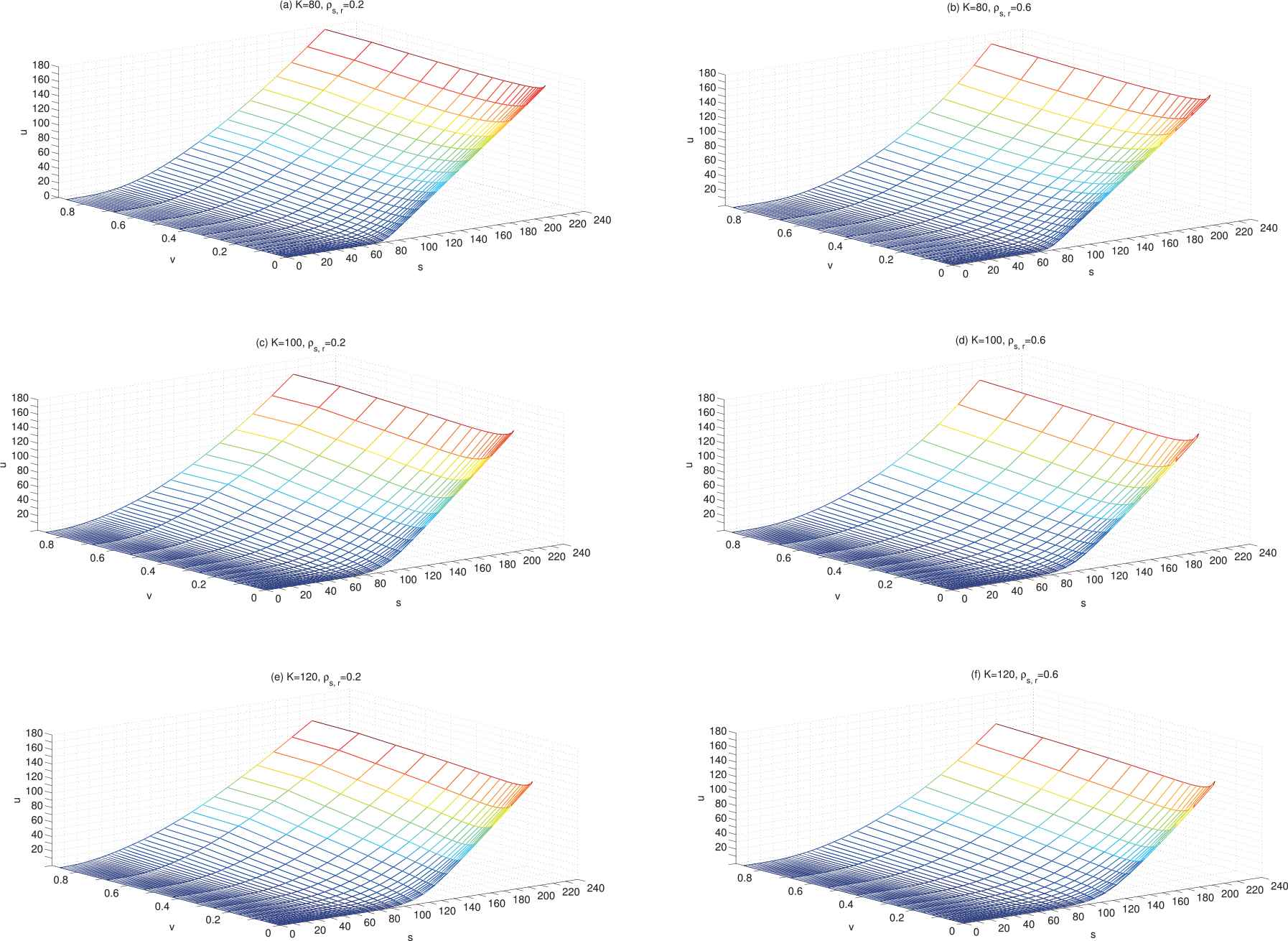
These parameters employed by Grzelak and Oosterlee [16]. Note that the Feller condition is not satisfied for this set of parameters, see Section 2 for details. We use the computation domain is [0,smax]×[0,νmax]×[0,rmax]=[0,240]×[0,0.9]×[0,0.9]. We approximated the exact option prices by FD discretization with Ns=2Nν=2Nr=40 and applying our method with Nt=3200 time steps. Figure 1 displays the European call option price functions u corresponding to the set of parameters A on the domain (s,ν)∈[0,240]×[0,0.9] with r = 0.02, for the several values of the strike prices K = 80, 100, 120 and the correlations ρs,r=0.2,0.6. As it is seen in the Figure 1, when the strike price is decreased, the call option prices will rise. This is obviously because a call option profit is equal to sT−K, so that, when the strike price is decreased, the call option profit will increase and this will lead to an increase in the call option price. In addition, this Figure demonstrated that the higher correlation ρs,r leads to lower call option prices. Therefore, the value of ρs,r affects the call option price.
Figure 1
Approximated European call option prices vs. (s, ν) for parameter set A with the interest rate r = 0.02, the number of time steps Nt=3200,, and the several values of strike price K = 80, 100, 120 and the correlations ρs,r=0.2,0.6.
The second set of parameters, set B, is as follows:
These parameters employed by Haentjens [17] in case I of Table 1, where the Feller condition is satisfied for the volatility process and the interest rate process. Here, the computation domain is [0,smax]×[0,νmax]×[0,rmax]=[0,200]×[0,0.9]×[0,0.9]. And the spatial grid is chosen to be Ns=2Nν=2Nr=40 with the number of time steps Nt=3200.
r
0.0222
0.0303
0.0685
0.0886
0.0222
1.0002
2.4616
5.1460
6.6989
0.0527
1.4283
3.7519
7.7441
9.7733
ν
0.0886
1.8376
4.9715
10.2205
12.7203
0.1470
2.4137
6.5366
13.7373
16.8908
0.2430
3.1345
8.4997
18.1068
20.0046
Table 1
European call option price as a function of ν and r, for parameter set B with K = 90 and s = 100.
Using this set of parameters, our numerical results for two strike price values k = 90, 100, and the various values of ν and r are presented in “Table 1” and “Table 2.” According to these tables, there will be an increase in call option price with the increase in volatility or interest rate. Therefore, it can be concluded that the call option price is affected by volatility and interest rate values. In other words, call option price is a function of volatility and interest rate.
r
0.0222
0.0303
0.0685
0.0886
0.0222
0.8972
2.1767
4.5657
6.0199
0.0527
1.3749
3.3881
7.4590
8.8560
ν
0.0886
1.8313
4.5415
10.2154
11.7044
0.1470
2.3619
6.0155
13.3945
15.4611
0.2430
3.0148
7.8452
17.3565
18.9505
Table 2
European call option price as a function of ν and r, for parameter set B with K = 100 and s = 100.
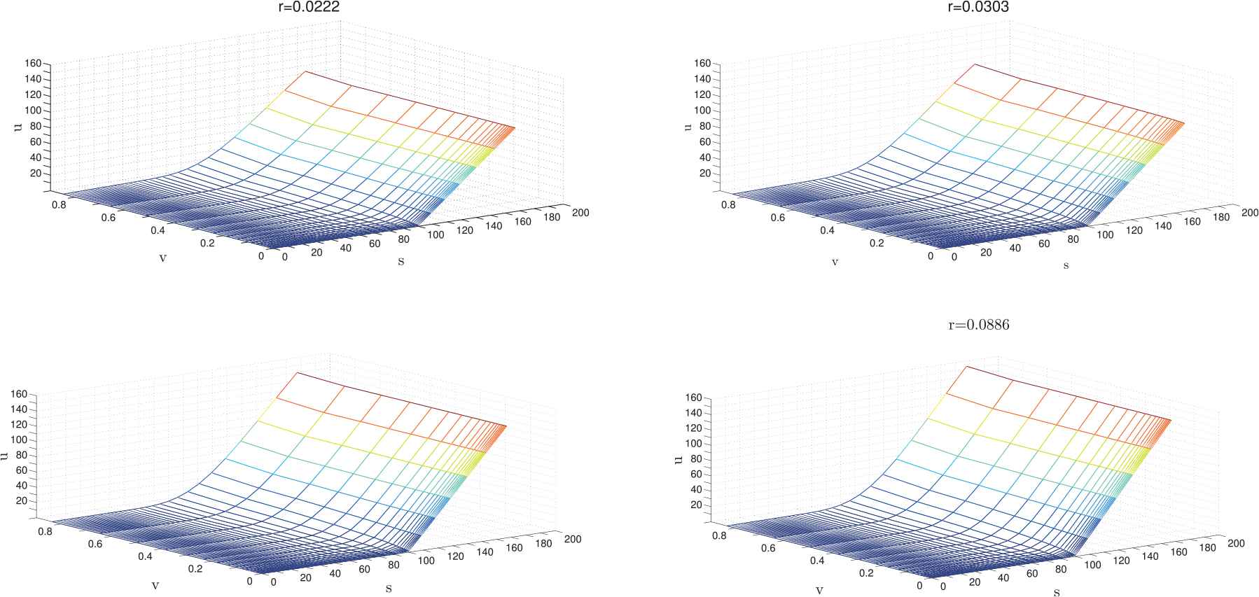
Figure 2 displays the European call option price functions u corresponding to the set of parameters B on the domain (s,ν)∈[0,200]×[0,0.9] with K = 100, for the various values of r = 0.0222, 0.0303, 0.0685, 0.0886. Figure 2 approves the fact that an increase in interest rate causes an increase in call option price.
Figure 2
Approximated European call option prices vs. (s, ν) for parameter set B with K = 100 and the various value of interest rate (a) r = 0.0222, (b) r = 0.0303, (c) r = 0.0685, (d) r = 0.0886.
This same direction between interest rate and call option price is due to the fact that if there is an increase in the interest rate, there will be an increase in the payoff and underlying asset price. Therefore, at the maturity time of call options, the underlying asset price will be higher than its previous price. And since a call option profit is equal to sT−K, when the value of s is increased (due to an increase in interest rate), the value of call option profit will increase and this will lead to an increase in call option price. Therefore, if there is an increase in interest rate, there will be an increase in call option price.
5.2. Comparison with Other Methods
Surely, the obtained numerical results by our proposed scheme are viable when compared with numerical results already given in the literature, or compared with some criterion. But, there is no quite reliable methods for three-factor models, see [33]. Furthermore, the exact solution to the HCIR PDE are not available in the literature, see [17]. Medvedev and Scaillet [34] have presented an analytical approximation to the prices of the put options in HCIR model. We now validate the option pricing method from this paper by comparing its results with the results given in [34].
The third set, set C, of parameters is the same as in [34] for comparison purpose:
Here, the computation domain is [0,smax]×[0,νmax]×[0,rmax]=[0,200]×[0,0.9]×[0,0.9].
Using this set of parameters, we first compute European put option prices by implementing the generalization of componentwise splitting method (GCS) presented in Section 4 and compare them with the solutions from Medvedev and Scaillet [34] using Monte-Carlo (MC) approach and the closed-form (c-f) formula. The results are presented in “Table 3” (for T = 0.25) and “Table 4” (for T = 0.5), for s = 100, ν=0.04, r = 0.04, and several values of K = 90, 100, 110. In these tables the numbers (Ns,Nν,Nr,Nt) denote the number of grid points. “Table 3” and “Table 4” show that our option prices are nicely with the ones reported in [34].
GCS = generalization of componentwise splitting method; MC = Monte-Carlo.
Table 4
European put option prices, for parameter set C, compared with reference values at s = 100, ν=0.0.4, r=0.04, and T = 0.50.
“Table 5” has the following columns: (Ns,Nν,Nr,Nt) defines the numbers of steps of the grid; RMSRD denotes the error column gives the root mean square relative differences; ratio gives the meaning of convergence ratio; and the last column gives the CPU times in seconds of our approach. For the results in the table, the error column gives the root mean square relative differences (RMSRD) are described in [35,36], for example. Moreover, the associated convergence rates (denoted by “ratio”) are calculated by dividing the error of the previous coarser time discretization by the error of the current discretization. “Table 5” suggest that GCS method improves the accuracy for larger of space and time steps. Moreover, we can observe from in Table that the discretizations appears to be roughly first-order accurate as the ratio values are 1.61 and 1.98 on average. From in Table, it can be observed that CPU time increase as the number of spatial discretization grids increases.
GSM-MC
GSM-c-f
grid(Ns,Nν,Nr,Nt)
RMSRD
ratio
RMSRD
ratio
CPU
(40, 20, 20, 80)
3.22×10⁻³
3.11×10⁻³
1.11
(60, 30, 30, 120)
1.29×10⁻³
2.50
1.09×10⁻³
2.85
5.46
(90, 45, 45, 180)
1.04×10⁻³
1.24
6.77×10⁻⁴
1.61
39.03
(100, 50, 50, 200)
9.46×10⁻⁴
1.10
3.83×10⁻⁴
1.76
69.32
MC = Monte-Carlo.
Table 5
The errors, the ratios of consecutive errors, and the CPU times in seconds, for parameter set C with s = 100, ν=0.0.4, r=0.04, and T = 0.50.
6. CONCLUSIONS
In this paper, we generalized a componentwise splitting method for pricing European call options by using the HCIR model. In this method, each time step was divided into six fractional time steps. In these six fractional time steps, the HCIR three-dimensional partial differential equation was decomposed into six one-dimensional equations. Then, each of these equations were represented in a tridiagonal system, each of which was solved by the Thomas algorithm.
The numerical experiments demonstrated that the European call option price was affected by the strike price, volatility, interest rate, and correlation ρs,r. So that, a decrease in the strike price or correlation ρs,r causes an increase in the call option price. On the other hand, an increase in volatility or interest rate causes an increase in the call option price. Furthermore, our numerical experiments showed that the computed prices are in agreement with the reference results discussed earlier.
In addition, the HCIR model has additional parameters (κ,η,ν¯,λ,γ,r¯,ρs,ν,ρs,r,ρν,r) compared to the Black-Scholes model. One needs to estimate the parameters to apply the model in practice. It should be noted that there is an inverse problem which works very well for the estimation procedure is given in Neisy and Salmani [37]. Applying the inverse problem to estimate the parameters of the HCIR model is part of our future plan.
3.J.P. Fouque, G. Papanicolaou, and K.R. Sircar, Derivatives in Financial Markets with Stochastic Volatility, Cambridge University Press, Cambridge, 2000.
18.N.N. Yanenko, The Method of Fractional Steps, The Solution of Problems of Mathematical Physics in Several Variables, Springer, Berlin Heidelberg, New York, 1971.
19.F.H.C. Naber, Fast solver for the three-factor Heston-Hull-White problem, Wholesale Banking Amsterdam ING, Amesterdam, 2007. PhD thesis
21.A.B. Vag, Pricing put options using Heston's stochastic volatility model, Norwegian University of Science and Technology, Norwegian, 2013. PhD thesis
22.A. Jiang, American spread option pricing with stochastic interest rate, Brigham Young University, Provo, 2016. PhD thesis
TY  - JOUR
AU  - Maryam Safaei
AU  - Abodolsadeh Neisy
AU  - Nader Nematollahi
PY  - 2019
DA  - 2019/12/17
TI  - Generalized Componentwise Splitting Scheme For Option Pricing Under The Heston-Cox-Ingersoll-Ross Model
JO  - Journal of Statistical Theory and Applications
SP  - 425
EP  - 438
VL  - 18
IS  - 4
SN  - 2214-1766
UR  - https://doi.org/10.2991/jsta.d.191209.001
DO  - 10.2991/jsta.d.191209.001
ID  - Safaei2019
ER  -