
Analysis of Count Data by Transmuted Geometric Distribution
- DOI
- 10.2991/jsta.d.191218.001How to use a DOI?
- Keywords
- Transmuted geometric distribution; EM algorithm; Likelihood Ratio test; Rao score's test; Wald's test
- Abstract
Transmuted geometric distribution (
- Copyright
- © 2019 The Authors. Published by Atlantis Press SARL.
- Open Access
- This is an open access article distributed under the CC BY-NC 4.0 license (http://creativecommons.org/licenses/by-nc/4.0/).
1. INTRODUCTION
Chakraborty and Bhati [1] recently introduced the transmuted geometric distribution
2. TRANSMUTED GEOMETRIC DISTRIBUTION (TGD (q, α))
A random variable (rv)
The corresponding survival function (sf) is written as
For
For
For
For
The probability generating function (PGF) of
The
where
3. RELIABILITY PROPERTIES AND STOCHASTIC ORDERING
There are several situations in reliability where continuous time is not a good scale to measure the lifetime, in production we may be interested in how many units are produced by the machine before failure or health insurance companies are interested how long a patient stays in hospital before discharge/death. In such situations, the discrete hazard rate functions can be used to model ageing properties of discrete random lifetimes. The different hazard rate functions of
3.1. Reliability Properties
3.1.1. Hazard rate function and its classification
The hazard rate function
The hazard rate function of
Hazard rate function plots of TGD(q, α).
Theorem 1.
The
Proof.
The hazard rate function of
But
Remark.
The hazard rate of
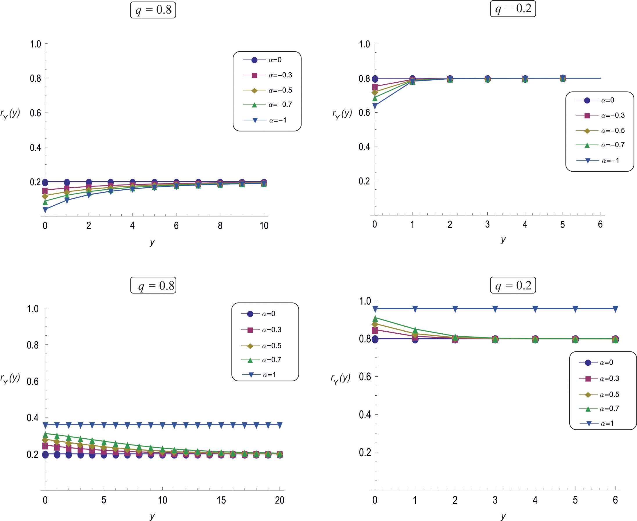
3.1.2. Mean residual life
Kemp (2004) presented various characterization of discrete lifetime distribution among them the mean residual life (MRL) or life expectancy is an important characteristic, for
Theorem 2.
The MRL function given in (3) is monotone decreasing (increasing) function of
Proof.
It can be easily be seen that
For any choice of
3.2. Stochastic Ordering
Many times there is a need of comparing the behavior of one rv with the other. Shaked and Shanthikumar [3] has given many comparisons such as likelihood ratio order
Theorem 3.
Let
Proof.
Since
Corollary.
Following results are direct implications of Theorem 3.
Theorem 4.
Let
Proof.
We know that
Hence
4. PARAMETER ESTIMATION AND THEIR COMPARATIVE EVALUATION
Estimates of the parameters
4.1. From Sample Proportion of 1's and 0's
If
4.2. From Sample Quantiles
If
4.3. Methods of Moments
Denoting the first and second observed raw moments by
Either solving the following two equations simultaneously
or by the minimization method proposed by Khan et al. [4] by minimizing
4.4. ML Method
Let
The MLE
4.5. MLE through EM Algorithm
The Expected Maximization (EM) algorithm is an useful iterative procedure to compute ML estimators in the presence of missing data or assumed to have a missing values. The procedure follows with two steps called Expectation step (E-Step) and Maximization step (M-Step). The E-step concerns with the estimation of those data which are not observed whereas the M-step is a maximization step for more details one may refer Dempster et al. [5]. Moreover, theorem 3.1 of Redner and Walker [6] ensures the consistency and uniqueness of the estimates obtained by EM procedure.
Let the complete-data be constituted with observed set of values
Under the formulation, the E-step of an EM cycle requires the expectation of
For M-step: The likelihood function of joint pmf of hypothetical complete-data
The components of the score function
The EM cycle will completed with the M-step by using the MLE over
4.5.1 Standard errors of estimates obtained from EM algorithm
In this section, we obtain the standard errors (se) of the estimators from the EM algorithm using result of Louis [8]. Let
Taking the conditional expectation of
Finally, the observed information matrix
4.6. Simulation Study to Evaluate EM Algorithm
Here we study the behavior of ML estimators obtained by direct numerical optimization and also through EM algorithm for different finite sample sizes and for different
| MLE |
EM Algorithm |
|||||||||
|---|---|---|---|---|---|---|---|---|---|---|
| Parameters | bias( |
bias( |
se( |
se( |
bias( |
bias( |
se( |
se( |
||
| 25 | −0.5566 | 0.0099 | 1.5154 | 0.1144 | −0.0132 | 0.0232 | 0.9739 | 0.1147 | ||
| 50 | −0.2675 | 0.0101 | 0.9151 | 0.0866 | −0.0081 | 0.0122 | 0.7215 | 0.0835 | ||
| 75 | −0.1733 | 0.0050 | 0.6880 | 0.0694 | −0.0049 | 0.0073 | 0.5881 | 0.0677 | ||
| 100 | −0.1327 | 0.0053 | 0.5780 | 0.0600 | −0.0035 | 0.0052 | 0.5137 | 0.0589 | ||
| 25 | −0.1348 | −0.0149 | 0.5644 | 0.0859 | −0.0031 | −0.0058 | 0.5664 | 0.0854 | ||
| 50 | −0.0077 | −0.0001 | 0.3960 | 0.0619 | 0.0012 | −0.0029 | 0.3888 | 0.0601 | ||
| 75 | −0.0196 | −0.0012 | 0.3197 | 0.0498 | −0.0006 | −0.0011 | 0.3155 | 0.0489 | ||
| 100 | −0.0113 | −0.0026 | 0.2765 | 0.0432 | 0.0012 | −0.0028 | 0.2730 | 0.0424 | ||
| 25 | −0.0411 | −0.0003 | 0.4012 | 0.0480 | 0.0060 | −0.0035 | 0.4190 | 0.0476 | ||
| 50 | −0.0085 | −0.0026 | 0.2766 | 0.0333 | −0.0002 | −0.0021 | 0.2964 | 0.0333 | ||
| 75 | −0.0011 | −0.0018 | 0.2242 | 0.0268 | 0.0012 | −0.0020 | 0.2337 | 0.0268 | ||
| 100 | −0.0008 | −0.0014 | 0.1909 | 0.0227 | −0.0009 | −0.0007 | 0.1990 | 0.0229 | ||
| 25 | −0.3455 | 0.0269 | 1.2484 | 0.1361 | −0.0340 | 0.0260 | 1.0043 | 0.1426 | ||
| 50 | −0.3055 | 0.0095 | 0.9006 | 0.1016 | −0.0240 | 0.0165 | 0.7203 | 0.1018 | ||
| 75 | −0.0391 | 0.0290 | 0.6466 | 0.0901 | −0.0125 | 0.0109 | 0.6045 | 0.0848 | ||
| 100 | −0.0997 | 0.0123 | 0.5770 | 0.0756 | −0.0090 | 0.0069 | 0.5269 | 0.0736 | ||
| 25 | −0.0310 | 0.0045 | 0.6288 | 0.1097 | −0.0037 | 0.0000 | 0.6840 | 0.1153 | ||
| 50 | −0.0249 | 0.0011 | 0.4672 | 0.0803 | −0.0031 | −0.0009 | 0.4818 | 0.0818 | ||
| 75 | −0.0253 | −0.0002 | 0.3880 | 0.0668 | −0.0029 | −0.0008 | 0.3908 | 0.0664 | ||
| 100 | −0.0258 | −0.0008 | 0.3375 | 0.0580 | −0.0036 | −0.0004 | 0.3333 | 0.0568 | ||
| 25 | −0.0503 | 0.0000 | 0.5182 | 0.0625 | −0.0010 | −0.0046 | 0.6044 | 0.0689 | ||
| 50 | −0.0432 | 0.0010 | 0.3850 | 0.0459 | 0.0069 | −0.0030 | 0.4157 | 0.0482 | ||
| 75 | −0.0020 | 0.0003 | 0.3141 | 0.0369 | −0.0038 | 0.0000 | 0.3324 | 0.0381 | ||
| 100 | −0.0009 | 0.0000 | 0.2838 | 0.0330 | −0.0026 | −0.0005 | 0.2899 | 0.0332 | ||
Note: EM = Expected Maximization; MLE = maximum likelihood estimator.
Average Bias and Average SE computed by method of maximum likelihood and EM Algorithm method.
4.6.1. Performance of estimators for different parametric values
A simulation study consisting of following steps is carried out for each triplet
Choose the value
Choose sample size
Generate
Compute the ML and EM estimate
Compute the average bias, standard error (SE) of the estimate.
In our experiment we have considered the number of replication
| MLE |
EM Algorithm |
|||||||||
|---|---|---|---|---|---|---|---|---|---|---|
| Parameters | bias( |
bias( |
se( |
se( |
bias( |
bias( |
se( |
se( |
||
| 25 | −0.4174 | 0.0254 | 1.1108 | 0.1524 | −0.1138 | −0.0206 | 0.7619 | 0.1547 | ||
| 50 | −0.2518 | 0.0178 | 0.8702 | 0.1281 | −0.0667 | −0.0158 | 0.8095 | 0.1632 | ||
| 75 | −0.1338 | 0.0193 | 0.6331 | 0.1110 | −0.0481 | −0.0144 | 0.6889 | 0.1386 | ||
| 100 | −0.0878 | 0.0215 | 0.5479 | 0.1013 | −0.0367 | −0.0032 | 0.6740 | 0.1353 | ||
| 25 | −0.2343 | 0.0226 | 0.5962 | 0.1328 | −0.0404 | −0.0267 | 0.7990 | 0.1700 | ||
| 50 | −0.1440 | 0.0184 | 0.4884 | 0.1085 | −0.0335 | −0.0354 | 0.6296 | 0.1349 | ||
| 75 | −0.0611 | 0.0142 | 0.4132 | 0.0926 | −0.0319 | −0.0336 | 0.5801 | 0.1237 | ||
| 100 | −0.0586 | 0.0125 | 0.3970 | 0.0886 | −0.0213 | −0.0210 | 0.5013 | 0.1072 | ||
| 25 | −0.0594 | 0.0127 | 0.5713 | 0.0829 | −0.0143 | −0.0326 | 0.7882 | 0.1101 | ||
| 50 | −0.0316 | 0.0097 | 0.4540 | 0.0652 | −0.0173 | −0.0508 | 0.6689 | 0.0923 | ||
| 75 | −0.0250 | 0.0079 | 0.3969 | 0.0568 | −0.0177 | −0.0607 | 0.5449 | 0.0759 | ||
| 100 | −0.0081 | 0.0050 | 0.3729 | 0.0522 | −0.0107 | −0.0224 | 0.5029 | 0.0691 | ||
| 25 | −0.0975 | 0.0038 | 0.0240 | 0.0042 | −0.0234 | −0.0305 | 0.6862 | 0.1166 | ||
| 50 | −0.0696 | 0.0138 | 0.0255 | 0.0027 | −0.0189 | −0.0220 | 0.5239 | 0.0423 | ||
| 75 | −0.0995 | 0.0046 | 0.0751 | 0.0038 | −0.0125 | −0.0112 | 0.4443 | 0.0259 | ||
| 100 | −0.0358 | 0.0070 | 0.0338 | 0.0027 | −0.0101 | −0.0071 | 0.4012 | 0.0125 | ||
| 25 | −0.1250 | 0.0288 | 0.5170 | 0.1474 | −0.0351 | −0.0112 | 0.5214 | 0.1627 | ||
| 50 | −0.1162 | 0.0248 | 0.4238 | 0.1186 | −0.0158 | −0.0131 | 0.4862 | 0.1456 | ||
| 75 | −0.0641 | 0.0140 | 0.3485 | 0.1000 | −0.0093 | −0.0583 | 0.3675 | 0.1088 | ||
| 100 | −0.0493 | 0.0125 | 0.3422 | 0.0974 | −0.0037 | −0.1109 | 0.6810 | 0.1963 | ||
| 25 | −0.1542 | 0.0350 | 0.5112 | 0.0966 | −0.0191 | −0.0176 | 0.5221 | 0.1048 | ||
| 50 | −0.1114 | 0.0178 | 0.4014 | 0.0727 | −0.0350 | −0.0253 | 0.4722 | 0.0858 | ||
| 75 | −0.0786 | 0.0100 | 0.3595 | 0.0638 | −0.1072 | −0.0986 | 0.3782 | 0.0676 | ||
| 100 | −0.0455 | 0.0100 | 0.3139 | 0.0566 | −0.1168 | −0.1178 | 0.3662 | 0.0647 | ||
Note: EM = Expected Maximization; MLE = maximum likelihood estimator.
Average Bias and Average SE computed by method of maximum likelihood and EM Algorithm method.
4.6.2 Performance of estimators for different sample size
In this subsection, we assess the performance of ML estimators of
Figures 2 and 3 show behavior of average bias and average standard error of parameter
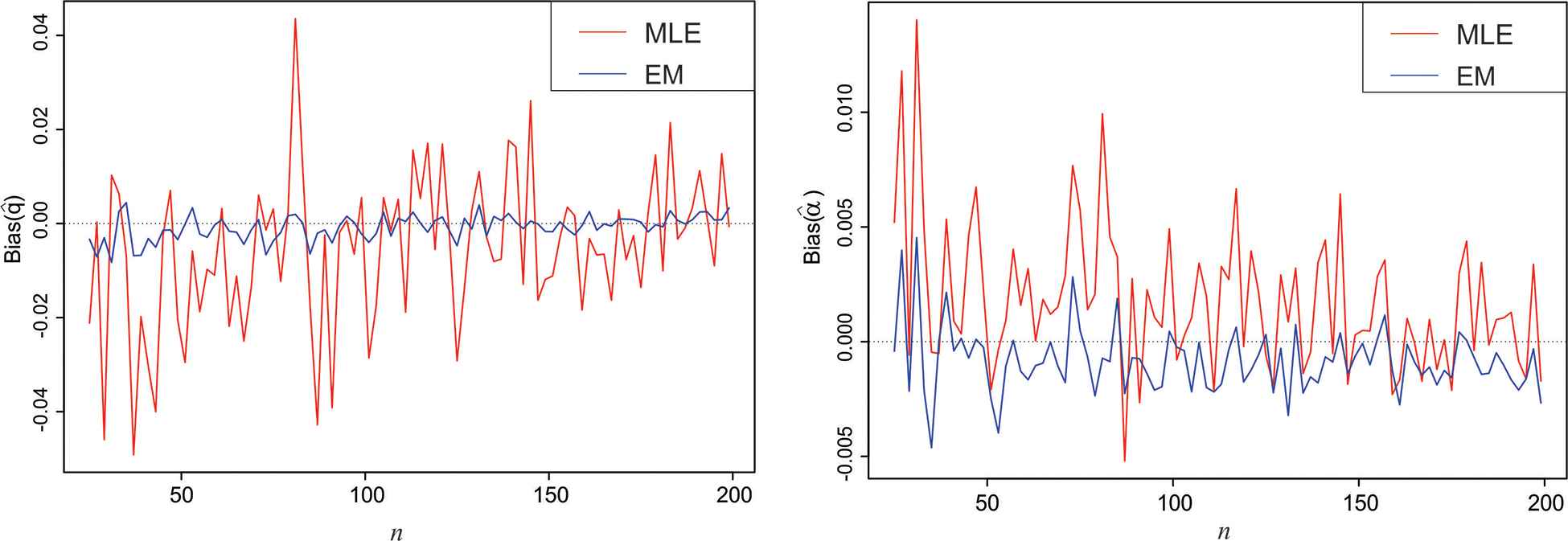
Bias plot of estimated value of parameter
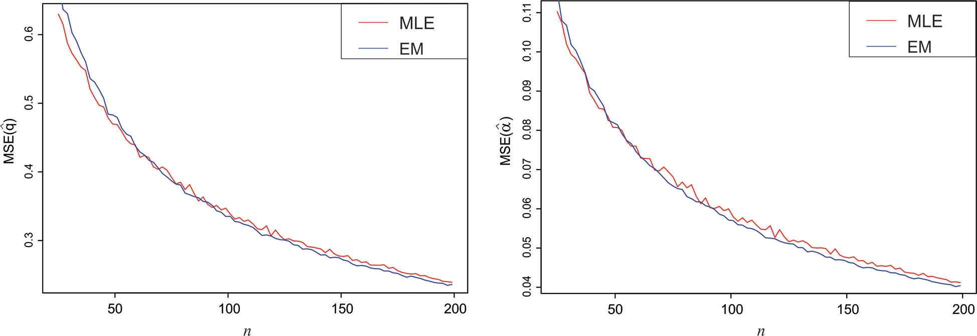
MSE plot of estimated value of parameter
Based on our findings it is clear that EM algorithm produces better ML estimators with smaller average bias as compared to the regular ML estimators while w.r.t. standard error there is not much to choose between the two procedures.
5. TESTS OF HYPOTHESIS
The
5.1. LRT, Rao's Score Test and Wald's Test
The LRT is based on the difference between the maximum of the likelihood under null and the alternative hypotheses. The LRT statistics is given by
The Rao's Score test [9] is based on the score vector defined as the first derivative of the LL function w.r.t. the parameters. Rao's score test statistic
The Wald's test statistics [10] is based on the difference between the maximum of the likelihood estimate value of the parameter under alternative hypothesis and the value of specified null hypothesis. The Wald's test statistic is given in our case by
All the test statistics follow asymptotically chi-square distribution with “
5.2. Statistical Power Analysis
Here we present a simulation based study of the statistical power of LR test, Rao's Score test and Wald's test considering
The power of the these test for different sample size, ES and for different parametric value
| q = 0.10 |
||||||||||||
|---|---|---|---|---|---|---|---|---|---|---|---|---|
| 100 |
300 |
500 |
1000 |
|||||||||
| LR | Score | Wald | LR | Score | Wald | LR | Score | Wald | LR | Score | Wald | |
| −0.7 | 0.028 | 0.051 | 0.042 | 0.117 | 0.066 | 0.017 | 0.252 | 0.133 | 0.01 | 0.476 | 0.351 | 0.087 |
| −0.5 | 0.02 | 0.046 | 0.041 | 0.052 | 0.039 | 0.029 | 0.121 | 0.066 | 0.024 | 0.237 | 0.134 | 0.015 |
| −0.3 | 0.022 | 0.081 | 0.056 | 0.024 | 0.032 | 0.037 | 0.059 | 0.035 | 0.034 | 0.101 | 0.045 | 0.019 |
| −0.1 | 0.013 | 0.11 | 0.066 | 0.02 | 0.069 | 0.061 | 0.036 | 0.045 | 0.046 | 0.059 | 0.04 | 0.032 |
| 0.1 | 0.015 | 0.173 | 0.074 | 0.021 | 0.123 | 0.109 | 0.042 | 0.112 | 0.099 | 0.058 | 0.105 | 0.071 |
| 0.3 | 0.009 | 0.239 | 0.091 | 0.026 | 0.209 | 0.143 | 0.038 | 0.212 | 0.161 | 0.079 | 0.237 | 0.134 |
| 0.5 | 0.005 | 0.28 | 0.112 | 0.041 | 0.351 | 0.217 | 0.069 | 0.394 | 0.266 | 0.142 | 0.431 | 0.288 |
| 0.7 | 0.033 | 0.262 | 0.132 | 0.025 | 0.452 | 0.236 | 0.074 | 0.523 | 0.336 | 0.197 | 0.602 | 0.436 |
| q = 0.30 |
||||||||||||
| 100 |
300 |
500 |
1000 |
|||||||||
| LR | Score | Wald | LR | Score | Wald | LR | Score | Wald | LR | Score | Wald | |
| −0.7 | 0.305 | 0.565 | 0.127 | 0.742 | 0.851 | 0.741 | 0.922 | 0.963 | 0.927 | 0.998 | 0.999 | 0.999 |
| −0.5 | 0.137 | 0.303 | 0.047 | 0.412 | 0.537 | 0.389 | 0.619 | 0.707 | 0.620 | 0.917 | 0.942 | 0.924 |
| −0.3 | 0.074 | 0.177 | 0.047 | 0.147 | 0.219 | 0.129 | 0.207 | 0.274 | 0.200 | 0.457 | 0.519 | 0.462 |
| −0.1 | 0.049 | 0.098 | 0.064 | 0.059 | 0.076 | 0.065 | 0.065 | 0.076 | 0.053 | 0.089 | 0.109 | 0.085 |
| 0.1 | 0.041 | 0.072 | 0.086 | 0.052 | 0.055 | 0.101 | 0.056 | 0.054 | 0.060 | 0.080 | 0.071 | 0.051 |
| 0.3 | 0.034 | 0.090 | 0.129 | 0.082 | 0.101 | 0.151 | 0.153 | 0.156 | 0.180 | 0.296 | 0.292 | 0.202 |
| 0.5 | 0.043 | 0.153 | 0.172 | 0.139 | 0.213 | 0.271 | 0.289 | 0.336 | 0.347 | 0.546 | 0.575 | 0.455 |
| 0.7 | 0.276 | 0.181 | 0.468 | 0.265 | 0.300 | 0.555 | 0.367 | 0.424 | 0.627 | 0.634 | 0.642 | 0.725 |
| q = 0.45 |
||||||||||||
| 100 |
300 |
500 |
1000 |
|||||||||
| LR | Score | Wald | LR | Score | Wald | LR | Score | Wald | LR | Score | Wald | |
| −0.7 | 0.470 | 0.787 | 0.563 | 0.933 | 0.982 | 0.956 | 0.989 | 0.997 | 0.993 | 1.000 | 1.000 | 1.000 |
| −0.5 | 0.241 | 0.540 | 0.310 | 0.611 | 0.792 | 0.675 | 0.835 | 0.909 | 0.873 | 0.993 | 0.996 | 0.994 |
| −0.3 | 0.089 | 0.279 | 0.125 | 0.223 | 0.368 | 0.280 | 0.325 | 0.465 | 0.391 | 0.641 | 0.729 | 0.699 |
| −0.1 | 0.058 | 0.157 | 0.089 | 0.076 | 0.128 | 0.105 | 0.071 | 0.106 | 0.085 | 0.090 | 0.137 | 0.122 |
| 0.1 | 0.035 | 0.083 | 0.078 | 0.060 | 0.062 | 0.096 | 0.059 | 0.055 | 0.071 | 0.097 | 0.073 | 0.051 |
| 0.3 | 0.033 | 0.062 | 0.117 | 0.117 | 0.083 | 0.171 | 0.210 | 0.163 | 0.193 | 0.396 | 0.313 | 0.233 |
| 0.5 | 0.055 | 0.106 | 0.199 | 0.224 | 0.200 | 0.316 | 0.417 | 0.351 | 0.427 | 0.700 | 0.645 | 0.539 |
| 0.7 | 0.268 | 0.121 | 0.468 | 0.347 | 0.227 | 0.639 | 0.497 | 0.377 | 0.711 | 0.763 | 0.685 | 0.805 |
Note: LR = likelihood ratio.
Power of the LR, Score and Walds Test for different sample sizes
| q = 0.6 |
||||||||||||
|---|---|---|---|---|---|---|---|---|---|---|---|---|
| 100 |
300 |
500 |
1000 |
|||||||||
| LR | Score | Wald | LR | Score | Wald | LR | Score | Wald | LR | Score | Wald | |
| −0.7 | 0.628 | 0.888 | 0.760 | 0.985 | 0.997 | 0.996 | 1.000 | 1.000 | 1.000 | 1.000 | 1.000 | 1.000 |
| −0.5 | 0.281 | 0.630 | 0.434 | 0.745 | 0.875 | 0.825 | 0.920 | 0.962 | 0.947 | 0.997 | 0.998 | 0.998 |
| −0.3 | 0.120 | 0.351 | 0.213 | 0.273 | 0.457 | 0.364 | 0.453 | 0.627 | 0.550 | 0.748 | 0.830 | 0.802 |
| −0.1 | 0.045 | 0.178 | 0.113 | 0.070 | 0.139 | 0.110 | 0.081 | 0.125 | 0.108 | 0.109 | 0.180 | 0.150 |
| 0.1 | 0.042 | 0.103 | 0.108 | 0.046 | 0.054 | 0.097 | 0.072 | 0.046 | 0.078 | 0.113 | 0.080 | 0.057 |
| 0.3 | 0.043 | 0.077 | 0.141 | 0.143 | 0.082 | 0.195 | 0.267 | 0.165 | 0.208 | 0.450 | 0.358 | 0.257 |
| 0.5 | 0.064 | 0.089 | 0.202 | 0.252 | 0.172 | 0.350 | 0.481 | 0.336 | 0.415 | 0.784 | 0.689 | 0.583 |
| 0.7 | 0.265 | 0.083 | 0.485 | 0.392 | 0.188 | 0.667 | 0.563 | 0.387 | 0.741 | 0.817 | 0.697 | 0.863 |
| q = 75 |
||||||||||||
| 100 |
300 |
500 |
1000 |
|||||||||
| LR | Score | Wald | LR | Score | Wald | LR | Score | Wald | LR | Score | Wald | |
| −0.7 | 0.698 | 0.941 | 0.852 | 0.994 | 1.000 | 0.998 | 1.000 | 1.000 | 1.000 | 1.000 | 1.000 | 1.000 |
| −0.5 | 0.336 | 0.686 | 0.532 | 0.798 | 0.921 | 0.868 | 0.956 | 0.987 | 0.979 | 0.998 | 0.999 | 0.999 |
| −0.3 | 0.142 | 0.374 | 0.245 | 0.297 | 0.512 | 0.418 | 0.488 | 0.669 | 0.600 | 0.810 | 0.877 | 0.860 |
| −0.1 | 0.045 | 0.188 | 0.131 | 0.057 | 0.150 | 0.119 | 0.077 | 0.153 | 0.130 | 0.090 | 0.167 | 0.141 |
| 0.1 | 0.045 | 0.112 | 0.115 | 0.060 | 0.056 | 0.110 | 0.095 | 0.071 | 0.104 | 0.092 | 0.057 | 0.045 |
| 0.3 | 0.044 | 0.072 | 0.139 | 0.145 | 0.076 | 0.179 | 0.299 | 0.182 | 0.236 | 0.470 | 0.356 | 0.245 |
| 0.5 | 0.091 | 0.078 | 0.242 | 0.285 | 0.164 | 0.355 | 0.491 | 0.321 | 0.427 | 0.789 | 0.683 | 0.586 |
| 0.7 | 0.316 | 0.089 | 0.525 | 0.412 | 0.176 | 0.657 | 0.585 | 0.369 | 0.764 | 0.845 | 0.698 | 0.860 |
Note: LR = likelihood ratio.
Power of the LR, Score and Walds Test for different sample sizes
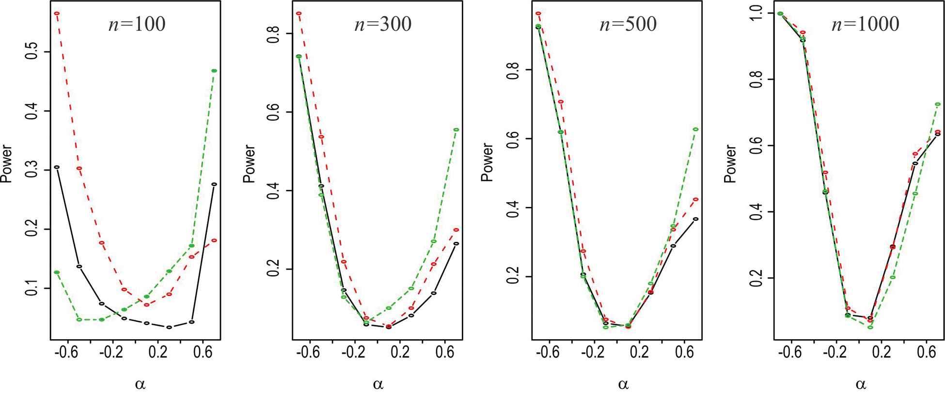
Power curve of likelihood ratio (LR) test (black), Score test (Red) and Wald's test (Green) for different n and q = 0.3.
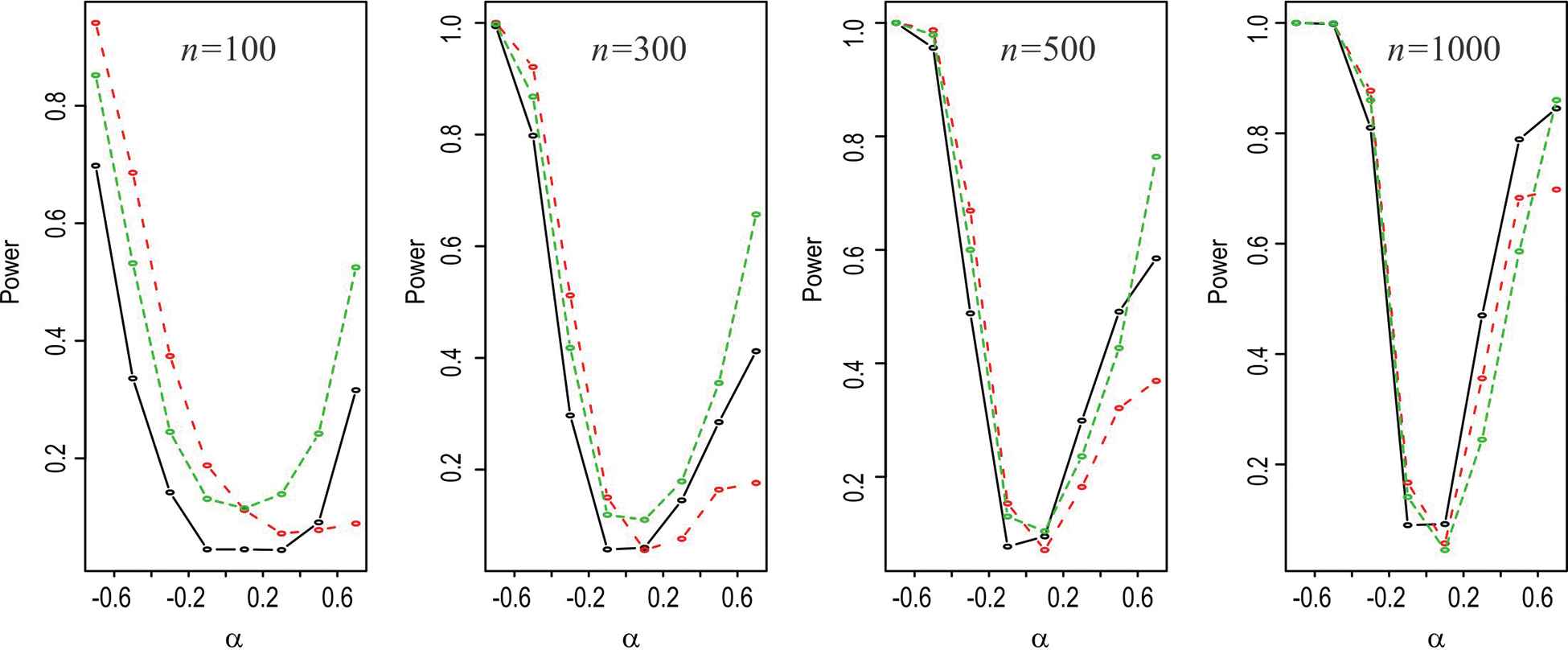
Power of likelihood ratio (LR) test (black), Score test (Red) and Wald's test (Green) for different n and q = 0.75.
6. DATA ANALYSIS
For the purpose of illustration, in this section, we consider following two data sets with details as follows:
Number of Fires in Greece (NTG)
The data comprise of numbers of fires in district forest of Greece from period 1 July 1998 to 31 August 1998. The observed sample values of size 123 for these data are the following (frequency in parentheses and none when it is equal to one): 0(16),1(13), 2(14), 3(9), 4(11), 5(13), 6(8), 7(4), 8(9), 9(6), 10(3), 11(4), 12(6), 15(4), 16, 20, 43. The data were previously studied by Bakouch et al. [11] and Karlis and Xekalaki [12].
Insurance Claim Count (ICC)
An insurance count data from Belgium in year 1993 is considered [13] and the data is as follows: 0(57178), 1(5617), 2(446), 3(50), 4(8).
The null hypothesis
| Data Set | Mean | Variance | LR test | Score Test | Wald's Test |
|---|---|---|---|---|---|
| NTG | 5.398 | 30.045 | 3.568 (0.059) | 41.018 (0.000) | 5.423 (0.020) |
| ICC | 0.106 | 0.115 | 9.178 (0.002) | 8.268 (0.004) | 8.118 (0.004) |
Notes: ICC = insurance claim count; LR = likelihood ratio; NTG = number of fires in Greece.
Descriptive and test statistic with p-value in parentheses for both the datasets.
| Dataset |
Model |
|||||
|---|---|---|---|---|---|---|
| NTG | Estimates | (0.802, 1.804) | (1.496, 0.223) | (2.470, 0.247) | (0.802, −0.531) | 0.839 |
| LL | −335.552 | −334.529 | −335.552 | −334.415 | −337.165 | |
| AIC | 675.104 | 673.058 | 675.104 | 672.830 | 676.330 | |
| BIC | 680.728 | 678.682 | 680.728 | 678.454 | 679.142 | |
| KS | 0.547 | 0.449 | 0.525 | 0.431 | 0.906 | |
| 0.767 | 0.882 | 0.847 | 0.899 | 0.432 | ||
| ICC | Estimates | (0.0845, 0.749) | (1.279, 0.924) | (5.870, 10.837) | (0.085, −0.157) | 0.095 |
| LL | −22063.8 | −22064.3 | −22063.8 | −22063.6 | −22068.2 | |
| AIC | 44131.6 | 44132.6 | 44131.6 | 44131.2 | 44138.4 | |
| BIC | 44149.7 | 44150.7 | 44149.7 | 44149.3 | 44147.4 | |
| KS | 0.091 | 0.102 | 0.091 | 0.074 | 0.427 | |
| 0.878 | 0.862 | 0.882 | 0.918 | 0.525 | ||
Notes: AIC = Akaiki Information Criteria; BIC = Bayesian Information Criteria; ICC = insurance claim count; LL = log likelihood; NTG = number of fires in Greece.
Comparative study of data fitting.
7. CONCLUSION
The current paper investigates some additional property of the
CONFLICT OF INTEREST
The authors declare they have no conflicts of interest.
Funding Statement
This research is not funded by any agency.
ACKNOWLEDGMENT
The authors acknowledge with thanks the comments of two anonymous referees which helped immensely in improving the presentation of the paper.
REFERENCES
Cite this article
TY  - JOUR
AU  - Subrata Chakraborty
AU  - Deepesh Bhati
PY  - 2019
DA  - 2019/12/27
TI  - Analysis of Count Data by Transmuted Geometric Distribution
JO  - Journal of Statistical Theory and Applications
SP  - 450
EP  - 463
VL  - 18
IS  - 4
SN  - 2214-1766
UR  - https://doi.org/10.2991/jsta.d.191218.001
DO  - 10.2991/jsta.d.191218.001
ID  - Chakraborty2019
ER  -