Some Applications of Near-Order Statistics in Two-Parameter Exponential Distribution

Masoumeh Akbari; Mahboubeh Akbari

doi:10.2991/jsta.d.200224.001

<Previous Article In Issue

Download article (PDF)

Next Article In Issue>

Volume 19, Issue 1, March 2020, Pages 21 - 27

Some Applications of Near-Order Statistics in Two-Parameter Exponential Distribution

Authors

Masoumeh Akbari¹^{, *}, Mahboubeh Akbari²

¹Department of Statistics, University of Mazandaran, Babolsar, Mazandaran 47416-95447, Iran

²Department of Statistics, University of Birjand, Birjand, 97175-615, Iran

^*Corresponding author. Email: m.akbari@umz.ac.ir

Corresponding Author

Masoumeh Akbari

Received 24 January 2017, Accepted 7 August 2017, Available Online 3 March 2020.

DOI: 10.2991/jsta.d.200224.001 How to use a DOI?
Keywords: Completeness properties; Exponential distribution; Müntz theorem; Near-order statistics
Abstract: In this paper, some characterization results for exponential distribution are established. The results are concluded in terms of number of observations near of order statistics. It is shown that its probability mass function and its first moment can characterize the exponential distribution. Also, an estimator based on near-order statistics is introduced for tail thickness of exponential distribution.
Copyright: © 2020 The Authors. Published by Atlantis Press SARL.
Open Access: This is an open access article distributed under the CC BY-NC 4.0 license (http://creativecommons.org/licenses/by-nc/4.0/).

1. INTRODUCTION

Two-parameter exponential distribution is the simplest lifetime distributions that is useable in survival analysis and reliability theory. So far, more results of characterization of exponential distribution have been obtained that some of them are based on order statistics. Let X1,X2,⋯Xn be independent and continuous random variables. The corresponding order statistics are the Xi's arranged in non-decreasing order, denoted by X1:n<X2:n<⋯<Xn:n. More details concerning order statistics can be seen in David and Nagaraja [1] and Arnold et al. [2]. Desu [3] proved that distribution of population is exponential if and only if nX1:n=dX1, for all n≥1, where the notation =d states the equality in distribution. Also, more characterization results of exponential distribution can be seen in Galambos and Kotz [4] and Ahsanullah and Hamedani [5]. Recently, the problem of number of observations near the order statistics is considered. At first, Pakes and Stutel [6] defined the number of observations within a of the sample maximum Xn:n as

Kn(a)=#{j=1,…,n,Xj∈(Xn:n−a,Xn:n]}.

Then, this definition was developed for the number of observations falling in the open left and right a–vicinity of the kth order statistics by Pakes and Li [7] and Balakrishnan and Stepanov [8], respectively. After that, following two random variables have been considered in the literature

K−(n,k,a)=#{j=1,…,n,Xj∈(Xk:n−a,Xk:n)},(1)

K+(n,k,a)=#{j=1,…,n,Xj∈(Xk:n,Xk:n+a)},(2)

where k=1,2,…,n and a>0 is a constant. So far, a lot of results for counting random variables in (1) and (2) have been obtained such that the most of them are focused on their asymptotic behavior under different conditions. For example, Pakes and Li [7], Balakrishnan and Stepanov [8,9], Dembińska et al. [10], Dembińska [11–14], Dembińska and Iliopoulos [15], Pakes [16–18] and Iliopoulos et al. [19]. There are few results of statistical inferences based on (1) and (2), for example, Müller [20] and Hashorva and Hüsler [21] considered the estimation of tails based on them. Also, some results have been obtained in terms of near-order insurance claims (See, e.g., Li and Pakes [22], Hashorva [23,24]).

In this paper, we will prove some characterization results of two-parameter exponential distribution based on these counting random variables which are stated in sections 2 and 3. An estimator of e−σa is introduced in section 4 and some properties of this estimator are discussed. Further, its performance is compared with the maximum likelihood estimator (MLE) through simulation.

2. CHARACTERIZATION BASED ON DISTRIBUTIONAL RESULTS

Let X be a random variable having two-parameter exponential distribution with parameters μ and σ, denoted by Exp(μ,σ). Then the cumulative distribution function (CDF) of X is

F (x)=1−e−σ(x−μ),x≥μ.(3)

According to (1), the probability mass function (pmf) of K+(n,k,a) for any j=0,1,⋯,n−k, have been obtained as (See Dembińska et al. [10])

P (K+(n,k,a)=j)=n!j!(k−1)!(n−k−j)!∫RF¯ n−k−j(x+a)(F¯ (x)−F¯ (x+a)) jF k−1(x)dF (x).(4)

Further, it is easy to verify that the pmf of K−(n,k,a) for any j=0,1,⋯,k−1 is

P (K−(n,k,a)=j)=n!j!(k−j−1)!(n−k)!∫RF k−j−1(x−a)(F (x)−F (x−a)) jF¯ n−k(x)dF (x).(5)

Now, assume that F(⋅) has a form as (3). Substituting in Eq. (4), we conclude easily that K+(n,k,a) has binomial distribution with parameters (n−k) and (1−e−σa), that is

P (K+(n,k,a)=j)=n−kje−σa(n−k−j)(1−e−σa) j,(6)

for any j=0,1,…,n−k. Therefore, the expected value of K+(n,k,a) is given by

E(K+(n,k,a))=(n−k)(1−e−σa).(7)

In this section, we will show that Eqs. (6) and (7) can characterize exponential distribution. The results are proved through properties of completeness sequence function. So, we firstly define complete sequence function and recall some well-known theorems.

Definition 2.1.

A sequence {Φn}n≥1 of elements of a Hilbert space H is called complete if the only element which is orthogonal to every {Φn} is the null element, that is,

〈 f,Φn〉⇒f=0,(8)

where 〈⋅,⋅〉 denotes the inner product of H. The Hilbert space L2(0,1) is considered here whose inner product is given by 〈 f,g〉=∫01f (x) g (x)dx, where f and g are two real-valued square integrable functions defined on (0,1).

The sequence {xn, n≥1} is the most important complete sequence function. Even under conditions a subsequence of it is a complete sequence that is stated in the following theorem and is well-known as the Müntz theorem.

Theorem 2.1.

Higgins ([25], p. 95) The set {xn1,xn2,⋯;1≤n1<n2<⋯} forms a complete sequence in L2(0,1) if and only if

∑j=1∞nj−1=∞.(9)

We refer the reader to Higgins [25] for Hilbert space and complete sequence function.

Theorem 2.2.

Let X1,X2,…,Xn be continuous random variables with CDF F. Then F has exponential distribution Exp(μ,σ) if and only if

P (K+(n,k,a)=j0)=(1−e−σa) j0,a>0,(10)

for a fixed j0∈{0,1,…,n−1} and k=n−j0.

Proof.

If X has exponential distribution, then Eq. (10) is easily obtain. Conversely, let (10) holds, then

0=P (K+(n,k,a)=j0)−(1−e−σa) j0.

From (4) we have

0=n!j0!(n−j0−1)!∫RF (x+a)−F (x) j0F n−j0−1(x)dF (x)−(1−e−σa) j0 =n!j0!(n−j0−1)!∫01(F (F −1(u)+a)−u) j0un−j0−1du −(1−e−σa) j0∫01n!j0!(n−j0−1)!un−j0−1(1−u) j0du =∫01(F (F −1(u)+a)−u) j0−(1−e−σa) j0(1−u) j0un−j0−1du.(11)

Taking η(u)=(F(F−1(u)+a)−u)j0, we have

∫01η2(u)du=∫01F (F −1(u)+a)−u2j0du≤1.

The above inequality shows that η(u)∈L2(0,1). Similarly we have the quantity

(1−e−σa) j0(1−u) j0∈L2(0,1).

Further, using Minkowski's inequality for the quantity

θ(u)={F (F −1(u)+a)−u} j0−(1−e−σa) j0(1−u) j0,

we get θ(u)∈L2(0,1). So, if (11) holds for any n≥j0+1, then using complete property of sequence {un−j0−1,n≥j0+1}, we have

{F (F −1(u)+a)−u} j0−(1−e−σa) j0(1−u) j0=0.(12)

From (12) is concluded that

F¯ (t+a)F¯ (t)=e−σa,a>0,t∈R,(13)

where t=F −1(u). The most general solution of (13) is the function F¯ (x)=ce−σx,x>0, where c is a constant. (See Aczél [26], pp. 17–18). Taking c=eσμ, the proof is completed.

The other characterization of exponential distribution is based on first moment of K+(n,k,a) which is stated in the next theorem.

Theorem 2.3.

Let X1,X2,…,Xn be continuous random variables with CDF F. Then F has exponential distribution Exp(μ,σ) if and only if for a fixed k≥1 and every a>0, following quantity holds.

E (K+(n,k,a))=(n−k)(1−e−σa),n≥k.

Proof.

If X has Exp(μ,σ), then from (7) proof of the necessity is concluded. Conversely, Let us assume that

E (K+(n,k,a))=(n−k)(1−e−σa).(14)

On the other hand, from (4) the first moment of K+(n,k,a) is given by

E (K+(n,k,a))=n−k−k(n−k)nk∫01F¯ (F −1(u)+a)uk−1(1−u)n−k−1du.(15)

The quantities (14) and (15) result in

knk∫01F¯ (F −1(u)+a)1−u−e−σauk−1(1−u)n−kdu=0.(16)

If Eq. (16) holds for any n≥k, then by completeness property of sequence {(1−u)n−k,n≥k}, we have

F¯ (F −1(u)+a)1−u−e−σauk−1=0.(17)

Similar to the proof of Theorem 2.2, F¯(x)=ce−σx is the most general solution of (17) and this completes the proof.

Remark 2.1.

According to Müntz theorem that is stated in Theorem 2.1, the all results of this section are true for any increasing subsequence {nj,j≥1} which satisfies in (9) instead of for all n≥1.

3. CHARACTERIZATION BASED ON DEPENDENCY ASSUMPTIONS

It is known that only for the exponential distribution, any two non-overlapping spacings will be independent (See, e.g., Arnold et al. [2]). Let us define two spacings W1 and W2 as follows

W1=Xk:n−Xk−j1:nandW2=Xk+j2:n−Xk:n,

for any j1=2,⋯,k−1 and j2=2,⋯,n−k. According to definitions K+(n,k,b) and K−(n,k,a), we can write the following equivalent events

K−(n,k,a)≤j1−1=W1≥a,

and

K+(n,k,b)≤j2−1=W2≥b.

So,

P (K−(n,k,a)≤j1−1)=P (W1≥a),(18)

and

P (K+(n,k,b)≤j2−1)=P (W2≥b).(19)

From (1) and (2), one can obtain easily the probability generating functions (pgf) of K−(n,k,a) and K+(n,k,b) as follows (see Balakrishnan and Stepanov [8])

Π−(n,k,a,s)=Es K−(n,k,a) =nn−1n−k∫{(1−s)F (x−a)+sF (x)}k−1{1−F (x)}n−kdF (x).(20)

Π+(n,k,b,t)=Et K+(n,k,b) =nn−1n−k∫t{F (x+b)−F (x)}+1−F (x+b)n−kF(x)k−1dF (x).(21)

It also follows that the joint pgf K−(n,k,a) and K+(n,k,b) is

Es K−(n,k,a)t K+(n,k,b)=nn−1n−k∫1−(1−s)F¯ (x−a)−sF¯ (x)k−1 ×(1−t)F¯ (x+b)+tF¯ (x)n−kdF (x).(22)

In the next theorem, we show an another characterization for exponential distribution based on independent near-order statistics.

Theorem 3.1.

Let X1,X2,…,Xn be continuous random variables with CDF F. Then F has Exp(μ,σ) if and only if K−(n,k,a) and K+(n,k,b) be independent for a fixed k≥1 and for any a>0 and b>0.

Proof of the necessity.

It is enough to show that joint pgf of K−(n,k,a) and K+(n,k,b) is equal with multiplication of their pgfs. Let F be Exp(μ,σ). Substituting it in Eqs. (20–22), we have

Π−E(n,k,a,s)=nn−1n−k∫e−σa1s k−1(1−u)k−1un−kdu +∫0e−σa{(1−s)(1−ueσa)+s(1−u)}k−1un−kdu,(23)

Π+E(n,k,b,t)=t(1−e−σb)+e−σbn−k,(24)

and

EEs K−(n,k,a)t K+(n,k,b)=nn−1n−k∫e−σa1(s−su)k−1(1−t)ue−σb+tun−kdu +∫0e−σa1−(1−s)ueσa−suk−1(1−t)ue−σb+tun−kdu.(25)

The above equality can be written as

EEs K−(n,k,a)t K+(n,k,b)=nn−1n−kΠ+E(n,k,b,t)∫e−σa1(s−su)k−1un−kdu +nn−1n−kΠ+E(n,k,b,t)∫0e−σa1−(1−s)ueσa−suk−1un−kdu =Π+E(n,k,b,t)Π−E(n,k,a,s),

and this completes the proof of necessity.

Proof of the sufficiency.

Suppose that counting random variables K−(n,k,a) and K+(n,k,b) be independent. Using (18) and (19), we have

P (W1≥a,W2≥b)=P (K−(n,k,a)≤j1−1,K+(n,k,b)≤j2−1) =P (K−(n,k,a)≤j1−1) P (K+(n,k,b)≤j2−1) =P (W1≥a)P (W2≥b).(26)

The quantity (26) shows that the spacings W1 and W2 are independent. So, the proof is completed.

4. AN ESTIMATOR BASED ON NEAR-ORDER STATISTIC

Pakes and Stutel [6] introduced following index of tail thickness when rF=inf{x,F(x)=1}=∞, as

γ(a)=limx→∞F¯ (x)−F¯ (x+a)F¯ (x).(27)

A tail is called as “thick” tail when γ(a)=0, “medium” tail when 0<γ(a)<1 and “thin” tail when γ(a)=1. Assume that X has exponential distribution. Substituting its CDF into (27), imply that

γ(a)=1−e−σa.(28)

It is well-known that the MLE of unknown scale parameter σ is n∑i=1n(Xi−X1:n)−1, when the underlying distribution is Exp(μ,σ). So, one estimator for e−σa based on MLE can be considered as

T1=exp−na∑i=1n(Xi−X1:n)−1.(29)

Following, we introduce an estimator for e−σa based on near-order statistic. From (6), the pmf of K+(n,k,a) can be written as

P (K+(n,k,a)=j)=n−kje−σa(n−k)ejlog1−e−σae−σa.(30)

Eq. (30) shows that the counting random variable K+(n,k,a) belongs to the one-parameter exponential family. Therefore, K+(n,k,a) is a sufficient and complete statistic for e−σa. According to expectation of K+(n,k,a), an unbiased estimator for e−σa is equal to

T2=1−K+(n,k,a)n−1.(31)

So, the estimator T2 is uniformly minimum-variance unbiased estimator (UMVUE) and its variance or minimum square error (MSE) is as follows

MSE (T2)=n−k(n−1)2(1−e−σa)e−σa.(32)

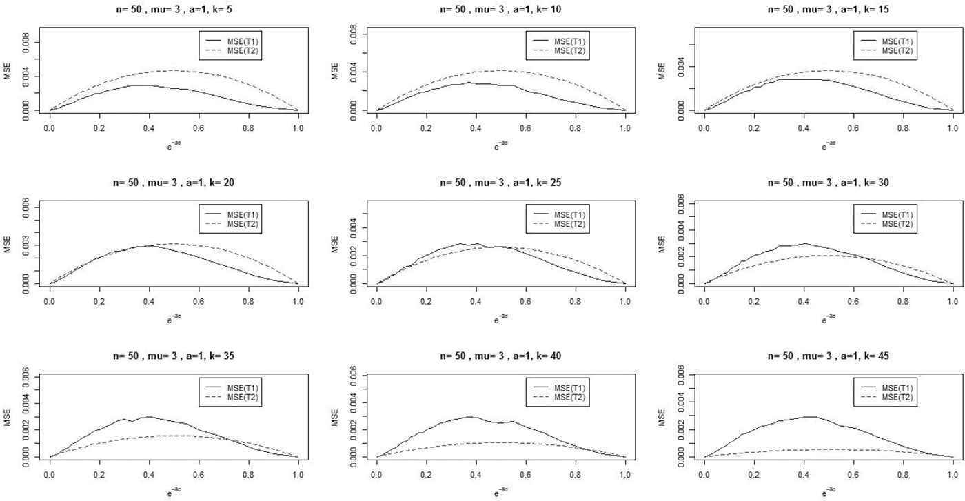
Further, (31) and (32) imply that T2 is a consistent estimator for e−σa. The performance of two estimators T1 and T2 is comparable through their MSE. But it is difficult to calculate MSE of T1 theoretically. So, we compare them numerically. In this study, we explore the MSE of T1 and T2 under different μ, a and k which are stated in Figure 1. Also, this results are obtained based on 2000 bootstrap samples.

Our simulation results demonstrate that the performance of T1 and T2 has little differences with increasing a.

So, the obtained results show that with choosing appropriate k, the estimator T2 can be considered as a good estimator for parameter e−σa.

An exact confidence interval for e−σa when a is known can be obtained by this fact that a confidence interval is available for σ in two-parameter exponential distribution. So, the 100(1−α)% interval confidence for e−σa is given by

exp−2aχ2n−2,α2 2∑i=1nXi−X1:n−1,exp−2aχ2n−2,1−α2 2∑i=1nXi−X1:n−1,

where χ(m,α) 2 denotes the 100(1−α)th percentile of the central chi-square distribution with m degree of freedom.

Now, we present an asymptotic confidence interval for e−σa based on counting random variable K+(n,k,a) which is stated in the following remark.

Remark 4.1.

According to distribution of K+(n,k,a), it can be considered as sum of independent and identically distributed random variables from binomial 1,1−e−σa. So the conditions of central limit theorem for random variable T2 hold and we have

(n−1)(T2−e−σa)(n−k)e−σa(1−e−σa)→dN(0,1).(33)

Therefor from (33), we can construct asymptotically confidence interval for e−σa by solving following inequality

e−2σaZα2 2+n−1−e−σaZα2 2+2(n−1)T2+(n−1)T2 2<0.

5. CONCLUSION

In this paper, we have shown some applications of counting random variable K+(n,k,a) for two-parameter exponential distribution. We believe that the results of the second and third section can be used in the construction of testing goodness-of-fit for exponentiality which sometimes can be more efficient or more robust than others. See, Nikitin [27] for more details on application of characterization in goodness-of-fit test.

CONFLICT OF INTEREST

The authors declare that there is no potential conflict of interest related to this study.

AUTHORS' CONTRIBUTIONS

The authors contributed equally to this work.

ACKNOWLEDGMENTS

The authors would like to thank the Editor in Chief, the Associate Editor and two anonymous reviewer for their valuable comments.

REFERENCES

1.H.A. David and H.N. Nagaraja, Order Statistics, John Wiley-Sons, New York, NY, USA, 2003.

2.B.C. Arnold, N. Balakrishnan, and H.N. Nagaraja, A First Course in Order Statistics, SIAM, Philadelphia, PA, USA, 2008.

3.M.M. Desu, Ann. Math. Stat., Vol. 42, 1971, pp. 837-838.

4.J. Galambos and S. Kotz, Characterizations of Probability Distributions, Springer-Verlag, New York, NY, USA, 1978.

5.M. Ahsanullah and G.G. Hamedani, Exponential Distribution—Theory and Methods, Nova Science Publications Inc., New York, NY, USA, 2009. https://books.google.com/books?id=BkcRRgAACAAJ

6.A.G. Pakes and F.W. Steutel, Aust. NZ. J. Stat., Vol. 39, 1997, pp. 179-193.

7.A.G. Pakes and Y. Li, Stat. Probab. Lett., Vol. 40, 1998, pp. 395-401.

8.N. Balakrishnan and A. Stepanov, J. Stat. Plan. Inf., Vol. 134, 2005, pp. 1-14.

9.N. Balakrishnan and A. Stepanov, J. Stat. Plan. Inf., Vol. 138, 2008, pp. 1010-1020.

10.A. Dembińska, A. Stepanov, and J. Wesolowski, Commun. Stat. Theor. Meth., Vol. 36, 2007, pp. 851-867.

11.A. Dembińska, Stat. Probab. Lett., Vol. 80, 2010, pp. 309-317.

12.A. Dembińska, J. Stat. Plan. Inf., Vol. 142, 2012, pp. 516-528.

13.A. Dembińska, Aust. NZ. J. Stat., Vol. 54, 2012, pp. 199-210.

14.A. Dembińska, Statistics, Vol. 48, 2014, pp. 508-523.

15.A. Dembińska and G. Iliopoulos, J. Multivariate Anal., Vol. 103, 2012, pp. 151-160.

16.A.G. Pakes, Adv. Appl. Math., Vol. 32, 2000, pp. 1100-1116.

17.A.G. Pakes, Extremes, Vol. 10, 2007, pp. 207-224.

18.A.G. Pakes, Aust. NZ. J. Stat., Vol. 54, 2009, pp. 375-395.

19.G. Iliopoulos, A. Dembińska, and N. Balakrishnan, Statistics, Vol. 46, 2012, pp. 85-97.

20.S. Müller, Methodol. Comput. Appl., Vol. 5, 2003, pp. 197-210.

21.E. Hashorva and J. Hüsler, Commun. Stat. Theor. Meth., Vol. 34, 2005, pp. 337-349.

22.Y. Li and A. Pakes, Insur. Math. Econ., Vol. 28, 2001, pp. 309-323.

23.E. Hashorva, Insur. Math. Econ., Vol. 32, 2003, pp. 37-49.

24.E. Hashorva, Stat. Probab. Lett., Vol. 69, 2004, pp. 117-128.

25.J.R. Higgins, Completeness and Basis Properties of Sets of Special Functions, Cambridge University Press, New York, NY, USA, 1977.

26.J. Aczél, Lectures on Functional Equations and Their Applications, Academic Press, London, England, New York, NY, USA, 1966.

27.Y. Nikitin, ACUTM, Vol. 21, 2017, pp. 3-24.

<Previous Article In Issue

Download article (PDF)

Next Article In Issue>

Journal: Journal of Statistical Theory and Applications
Volume-Issue: 19 - 1
Pages: 21 - 27
Publication Date: 2020/03/03
ISSN (Online): 2214-1766
ISSN (Print): 1538-7887
DOI: 10.2991/jsta.d.200224.001 How to use a DOI?
Open Access: This is an open access article distributed under the CC BY-NC 4.0 license (http://creativecommons.org/licenses/by-nc/4.0/).

Cite this article

ris enw bib

TY  - JOUR
AU  - Masoumeh Akbari
AU  - Mahboubeh Akbari
PY  - 2020
DA  - 2020/03/03
TI  - Some Applications of Near-Order Statistics in Two-Parameter Exponential Distribution
JO  - Journal of Statistical Theory and Applications
SP  - 21
EP  - 27
VL  - 19
IS  - 1
SN  - 2214-1766
UR  - https://doi.org/10.2991/jsta.d.200224.001
DO  - 10.2991/jsta.d.200224.001
ID  - Akbari2020
ER  -

download .riscopy to clipboard