
Bayes Factors for Comparison of Two-Way ANOVA Models
 , M. R. Srinivasan2
- DOI
- 10.2991/jsta.d.201230.001How to use a DOI?
- Keywords
- ANOVA model; Bayes factor; Zellner's g prior; Jeffrey-Zellner-Siow prior; Hyper-g prior; Simulation data
- Abstract
In the traditional two-way analysis of variance (ANOVA) model, it is possible to identify the significance of both the main effects and their interaction based on the P values. However, it is not possible to determine how much data supports the model when these effects are incorporated into the model. To overcome this practical difficulty, we applied Bayes factors for hierarchical models to check the intensity of the effects (both main and interaction). The objective is to identify the impact of the main and interaction effects based on a comparison of Bayes factors of the hierarchical ANOVA models. The application of Bayes factors enables to observe which model strengthens more while including or eliminating the effects in the model. Consequently, this paper proposes three priors such as Zellner's g, Jefferys-Zellner-Siow, and Hyper-g priors, to compute the Bayes factor. Finally, we extended this procedure to the simulation data for the generalization of the Bayesian results.
- Copyright
- © 2021 The Authors. Published by Atlantis Press B.V.
- Open Access
- This is an open access article distributed under the CC BY-NC 4.0 license (http://creativecommons.org/licenses/by-nc/4.0/).
1. INTRODUCTION
The Bayesian method is widely applied in a range of disciplines such as engineering, medicine, biology, economics, etc. Jeffrey [1] developed the Bayesian approach to solve hypothesis testing problems. He also developed a methodology for quantifying the evidence in favor of a scientific theory. Kass and Raftery [2] discussed the Bayesian viewpoints and several techniques for computing Bayes factor. Bayesian approach to the analysis of variance (ANOVA) model was discussed by many authors (Liang et al. [3]; Maruyama and George [4]; Wetzels et al. [5], etc.). In this study, we aim to identify the influence of the effects when we incorporate eliminating from the ANOVA two-way models by the Bayesian approach. The main advantage of this approach is that the evidence is quantified, instead of forcing an all or none decision as in the frequentist approach. The Bayes factor results are quantified in Table 1. Several priors are discussed to find the Bayes factor by many authors, Liang et al. [3], Wang and Sun [6], Kass and Raftery [2], Clyde et al. [7].
| Data Support the Model Mj if log(Bij) Value | Data Support the Model Mi if log(Bij) Value | Evidence for Respective Model |
|---|---|---|
| Decisive | ||
| −2 to −1 | 1 to 2 | Strong |
| −1 to −0.5 | 0.5 to 1 | Substantial |
| −0.5 to 0 | 0 to 0.5 | Poor |
Interpretations of Bayes factor.
1.1. Zellner's g Prior
Zellner's
1.2. Jeffrey-Zellner-Siow Prior
Jeffrey-Zellenr-Siow (JZS) prior is a mixture of priors, such that, Jeffreys' prior on the intercept and an inverse gamma with ½ and n/2 prior on g. Further, estimate
1.3. Hyper-g Prior
Hyper-
To avoid the ambiguous conclusions of the Bayesian approach, we propose three different priors such as Zellner's g, Jeffreys-Zellner-Siow, and Hyper-g priors, Wetzels et al. [5], Perrakis and Ntzoufras [10], Vijayaragunathan and Srinivasan [11]. The level of interpretations for the Bayes factor for the null and alternative model are in Table 1. The results are quantified evidence of data support the respective model, which was discussed extensively by Jeffreys [1] and Kass and Raftery [10].
2. ANOVA TWO-WAY MODELS AND BAYESIAN APPROACH
Factor A has a levels, a factor B has b levels, and these factors are arranged in a factorial design each replicate of the experiment contains all ab treatment combinations. An ANOVA two-factor experimental design is
The two-way ANOVA model is converted into a regression framework model for our convenience in applying the Bayesian technique to different priors Zellner et al. [13]. To test the outcome of main effects
The two-way ANOVA model containing only the main effects, without interaction effects, is
The two-way ANOVA model containing only the main effect
The two-way ANOVA model containing only the main effect
The two-way ANOVA model without main and interaction effects (the null model) is
Let
3. APPLICATIONS
Consider an engineer is designing a battery for use in a device that will be subject to some extreme variations in temperature, and he has three possible choices of plate material [14]. The engineer has no control over the temperature extremes that the device will encounter, and he knows from experience that temperature will probably affect the effectiveness of battery life. He decides that all three plate materials at three temperature levels (
| ANOVA | Main Effect A | Main Effect B | Interaction | R Square |
|---|---|---|---|---|
| Model 1 | 7.9114 (0.001976*) | 28.967 (1.9 × 10⁻⁷*) | 3.5595 (0.018611*) | 0.7652 |
| Model 2 | 5.947 (0.00651*) | 21.776 (1.24 × 10⁻⁶*) | – | 0.6414 |
| Model 3 | 2.633 (0.0869*) | – | – | 0.1376 |
| Model 4 | – | 16.75 (9.51 × 10⁻⁶*) | – | 0.5038 |
F ratio for four ANOVA models (* represents P values).
In the first step of the Bayesian approach, we have computed the Bayes Factor for all ANOVA models with the null model, to know how the data support the respective models. From Table 3, the evidence of data supports “decisively” for the two-way ANOVA models such as model 1 (full model), model 2 (except interaction effects model), and model 4 (only main effect
| Prior | BF10 | BF20 | BF30 | BF40 |
|---|---|---|---|---|
| UIP | 4.0987 | 4.2990 | −0.4759 | 3.5521 |
| RIC | 3.3896 | 4.3936 | 0.1874 | 3.2220 |
| JZS | 4.1908 | 4.1087 | −0.5450 | 3.3363 |
| Hyper-g(a = 3) | 4.2165 | 3.9933 | 0.0615 | 3.1474 |
| Hyper-g(a = 4) | 4.0314 | 3.7685 | 0.1466 | 2.9049 |
UIP, Unit Information Prior; RIC, Risk Inflation Criterion; JZS, Jeffrey-Zellenr-Siow.
Bayes factor for respective two-way ANOVA model with the null model.
The two-way ANOVA with interaction effect model (full model) is a larger model, other models are nested models to it, and so on. Now, to test the effect of interaction by comparing the full model and without the interaction model. In the same way, we used the without interaction model and respective main effect models to test the main effects. In general, the Bayes factors for the larger model to the nested model have been computed to know the strength of the effect which was eliminated in nested models.
The ratio of Bayes factors of the full model and without interaction models indicate that there is an intensity of the interaction effect in the model. The Bayes factor values are close to one for BF(12) and BF(24), which gives the impression that the data support “strongly” for both interaction and main effect
4. SIMULATION STUDY
In an examination of the effects of the two-way ANOVA model, we constructed the different datasets by varying different error variance in the simulation. To find the Bayes Factors for all priors, we have to simulate datasets to obtain reliable conclusions. Firstly, we simulated 1000 different data sets with variance 1 to compute the 1000 Bayes factor values for each prior. Similarly, we simulated the other two datasets with the error variances 10 and 25 to compute Bayes factors. These results are shown in Figures 1–5 and also display the summary statistics for the Bayes factor of respective simulation data to the ANOVA model are shown in Table 4–9. The overall conclusion of all the priors do not change in BF(12) and BF(24), but it varies in BF(23). Thus, our simulation study provides broad knowledge about the different priors of various datasets. Consequently, it may be useful to make decisions for inclusion or elimination of the interaction effect in the two-way ANOVA model as well as the influence of the main effects in the model.
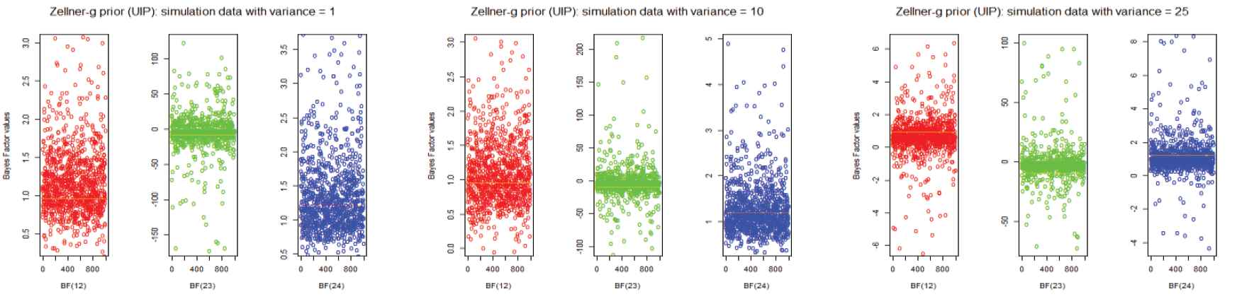
Bayes factors of simulation data sets for different variances to the Zellner's g prior (unit information prior).
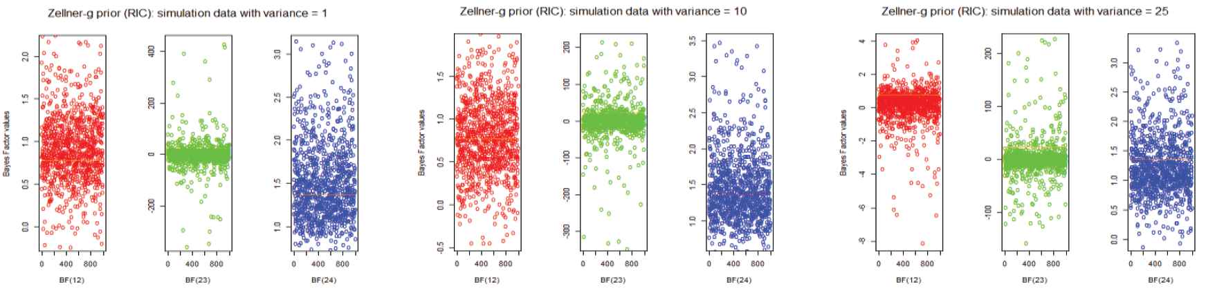
Bayes factors of simulation data sets for different variances to the Zellner's g prior (risk inflation criterion).
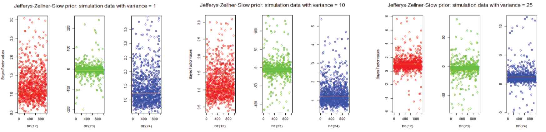
Bayes factors of simulation datasets for different variances to the Jeffreys-Zellner-Siow prior.
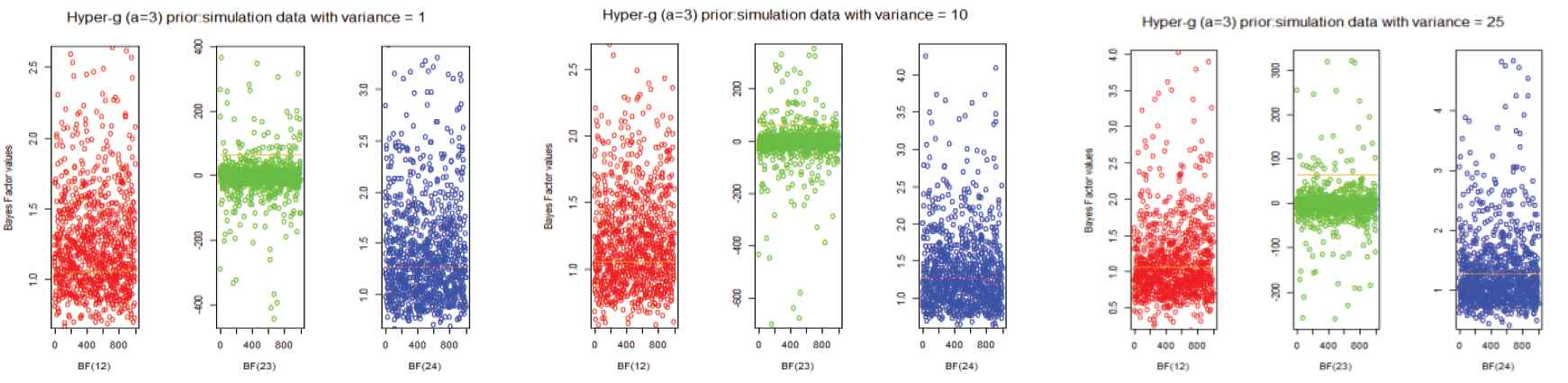
Bayes factors of simulation datasets for different variances to the hyper-g (a = 3) prior.
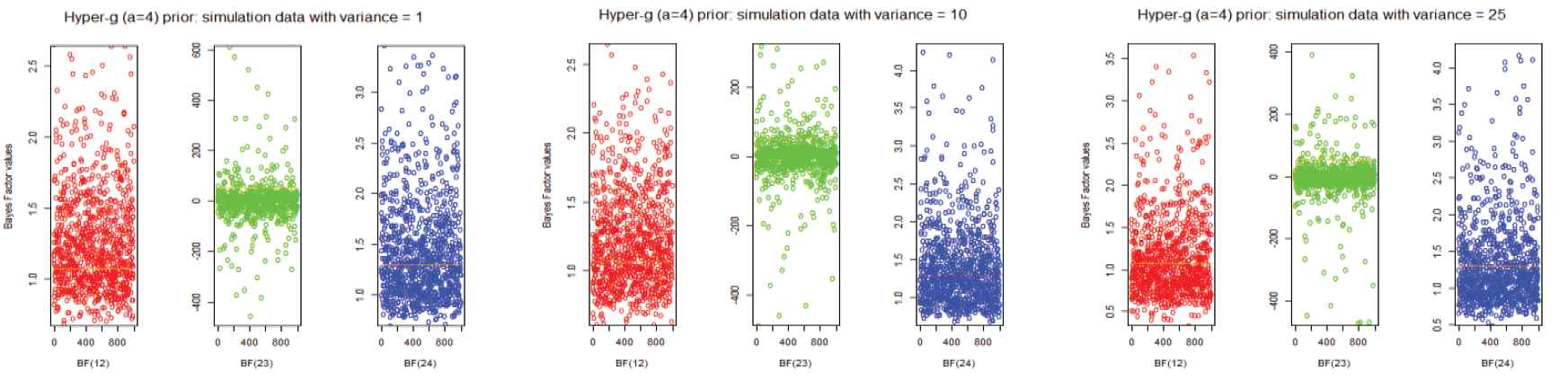
Bayes factors of simulation datasets for different variances to the hyper-g (a = 4) prior.
| Prior | BF12 | BF23 | BF24 |
|---|---|---|---|
| UIP | 0.9534 | −9.0334 | 1.2103 |
| RIC | 0.7715 | 23.4450 | 1.3636 |
| JZS | 1.0200 | −7.5389 | 1.2315 |
| Hyper-g(a = 3) | 1.0559 | 64.9317 | 1.2688 |
| Hyper-g(a = 4) | 1.0698 | 52.6239 | 1.2973 |
UIP, Unit Information Prior; RIC, Risk Inflation Criterion; JZS, Jeffrey-Zellenr-Siow.
Ratio of Bayes factors for the relevant ANOVA models.
| Error Variance | Descriptive |
BF12 |
BF23 |
BF24 |
|---|---|---|---|---|
| Actual | 0.95 | −9.03 | 1.21 | |
| 1 | Mean (SD) | 1.19 (0.49) | −7.10 (172.93) | 1.38 (0.61) |
| 10 | Mean (SD) | 1.05 (2.20) | −1.88 (77.78) | 1.51 (5.94) |
| 25 | Mean (SD) | 0.73 (3.91) | 1.51 (5.94) | 1.05 (2.83) |
Summary of Bayes factors for Zellner's g prior (unit information prior).
| Error Variance | Descriptive |
BF12 |
BF23 |
BF24 |
|---|---|---|---|---|
| Actual | 0.77 | 23.45 | 1.36 | |
| 1 | Mean (SD) | 0.92 (0.43) | −132.39 (4261.64) | 1.53 (0.48) |
| 10 | Mean (SD) | 0.79 (0.49) | −1.70 (173.45) | 1.48 (0.60) |
| 25 | Mean (SD) | 0.22 (3.99) | −5.83 (530.68) | 1.15 (1.80) |
Summary of Bayes factors for Zellner's g prior (risk inflation criterion).
| Error Variance | Descriptive |
BF12 |
BF23 |
BF24 |
|---|---|---|---|---|
| Actual | 1.02 | −7.54 | 1.23 | |
| 1 | Mean (SD) | 1.26 (0.46) | 1.24 (0.84) | 1.43 (0.69) |
| 10 | Mean (SD) | 1.24 (0.84) | −21.61 (417.78) | 1.28 (3.14) |
| 25 | Mean (SD) | 1.02 (2.17) | −4.55 (75.76) | 1.64 (8.01) |
Summary of Bayes factors for Jeffreys-Zellner-Siow prior.
| Error Variance | Descriptive |
BF12 |
BF23 |
BF24 |
|---|---|---|---|---|
| Actual | 1.06 | 64.93 | 1.27 | |
| 1 | Mean (SD) | 1.27 (0.38) | −9.88 (364.94) | 1.43 (0.54) |
| 10 | Mean (SD) | 1.23 (0.41) | −36.57 (733.52) | 1.42 (0.76) |
| 25 | Mean (SD) | 1.17 (0.85) | −16.17 (1.33) | 1.33 (1.01) |
Summary of Bayes factors for hyper-g (a = 3) prior.
| Error Variance | Descriptive |
BF12 |
BF23 |
BF24 |
|---|---|---|---|---|
| Actual | 1.07 | 52.62 | 1.30 | |
| 1 | Mean (SD) | 1.28 (0.37) | 32.36 (750.47) | 1.46 (0.55) |
| 10 | Mean (SD) | 1.25 (0.40) | 8.64 (281.79) | 1.45 (0.71) |
| 25 | Mean (SD) | 1.18 (0.67) | −6.58 (309.83) | 0.95 (14.07) |
Summary of Bayes factors for hyper-g (a = 4) prior.
5. CONCLUSIONS
An ANOVA is one of the most popularly used statistical tools in research. We considered a two-way ANOVA model consisting of two factors such as plate material
CONFLICTS OF INTEREST
The authors declare that they have no conflict of interest.
AUTHORS' CONTRIBUTIONS
Both the authors contributed equally and approved the final manuscript.
ACKNOWLEDGMENTS
The authors would like to thank the editor and the reviewers for their constructive comments and suggestions which highly improved the paper. Also, state that this research did not receive any specific grant from any funding agencies.
REFERENCES
Cite this article
TY  - JOUR
AU  - R. Vijayaragunathan
AU  - M. R. Srinivasan
PY  - 2021
DA  - 2021/01/05
TI  - Bayes Factors for Comparison of Two-Way ANOVA Models
JO  - Journal of Statistical Theory and Applications
SP  - 540
EP  - 546
VL  - 19
IS  - 4
SN  - 2214-1766
UR  - https://doi.org/10.2991/jsta.d.201230.001
DO  - 10.2991/jsta.d.201230.001
ID  - Vijayaragunathan2021
ER  -