
Transmuted Lower Record Type Fréchet Distribution with Lifetime Regression Analysis Based on Type I-Censored Data
- DOI
- 10.2991/jsta.d.210115.001How to use a DOI?
- Keywords
- Fréchet distribution; Lower records; Point estimates; Lifetime regression
- Abstract
This paper introduces a new lifetime distribution by mixing the first two lower record values and various distributional properties are examined. Statistical inference on distribution parameters are discussed with five estimators. A Monte Carlo simulation study is carried out to evaluate the risk behavior of these estimators for different sample of sizes. The distribution modeling analysis is provided based on real data to demonstrate the fitting ability of the proposed model. In addition, a lifetime regression model is described by re-parameterization on the log lifetimes. The superiority of proposed regression model is revealed in well-known models.
- Copyright
- © 2021 The Authors. Published by Atlantis Press B.V.
- Open Access
- This is an open access article distributed under the CC BY-NC 4.0 license (http://creativecommons.org/licenses/by-nc/4.0/).
1. INTRODUCTION
In two decades, many statistical distributions have been brought into the literature. These distributions are obtained as a member of the family of distributions. Transmuted families can be given as an example to the family of distributions. In general, transmuted families are given based on order statistics. The transmuted distributions has been introduced by Shaw and Buckley [1,2] using a quadratic transmutation map. Order statistics, transmuted distributions can be sorted as [3–5]. Recently, Balakrishnan [6] proposed a new record based transmuted family of distributions. Tanış and Saraçoğlu [7] examined a special model based on Weibull distribution of record based transmuted family of distributions. In terms of both distributional properties and statistical inference, in parallel with the study of [6].
In our study, we obtained the transmuted version of the Fréchet distribution based on lower record values. In Section 2, a transmutation lower record type map of order 2 is introduced. In Section 3, we have suggested a sub-model called transmuted lower record type Fréchet (TLRT-F) distribution and the some distributional properties are obtained such as moments, incomplete moments, Bonferroni and Lorenz curves. In Section 4, the unknown parameters are estimated by five methods including maximum likelihood estimators, least squares estimators, weighted least squares estimators, Anderson-Darling estimators, and Cramer von-Mises estimators. A simulation study is performed in order to compare the performance of these estimators in terms of mean squared errors (MSEs) and bias. A lifetime regression is introduced based on TLRT-F distribution in Section 5. In Sections 6 and 7, two applications with real data are presented to show the applicability of introduced distribution.
2. TRANSMUTATION LOWER RECORD TYPE MAP OF ORDER 2
Let
It is noticed that the distribution with cdf (2.2) is called “transmuted lower record type distribution (TLRT).” Using (2.2), the probability density function (pdf) and hazard function(hf) of TLRT distribution are given by
3. TLRT-F DISTRIBUTION AND DISTRIBUTIONAL PROPERTIES
In this section, we investigate the sub-model of TLRT family. Let
The hf of TLRT-F distribution is given by
Figures 1–2 illustrates the possible shapes of pdf and hf for selected parameters. The quantile function of the TLRT-F is given by
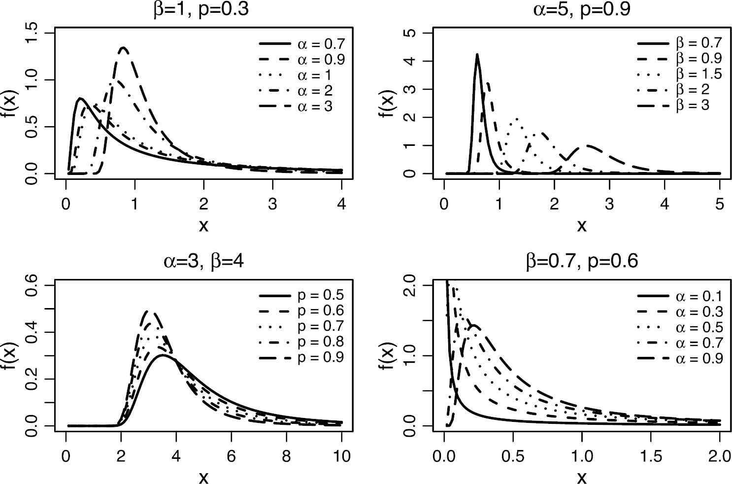
The probability density function plots for transmuted lower record type Fréchet (TLRT-F) distribution.
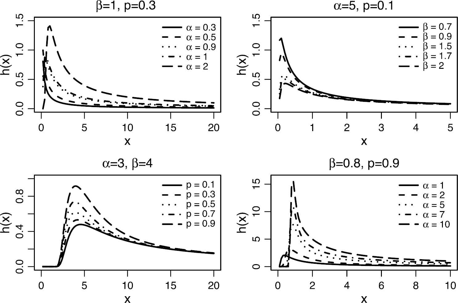
The hazard function plots of transmuted lower record type Fréchet (TLRT-F) distribution.
For
The incomplete moments of TLRT-F distribution is obtained by
The Bonferroni and Lorenz curves for TLRT-F are given, respectively, by
Stochastic and the other ordering are important means for evaluating the comparative properties for a positive continuous random variable. The following theorem shows that the TLRT-F random variables can be ordered with respect to the likelihood ratio.
Theorem 3.1.
Let
Proof.
For any
Consider the derivative of
Corollary 3.1.
It follows from [8] that
In order to generate the data from TLRT-F distribution, an acceptance-rejection (AR) sampling method is given in the following algorithm. In this algorithm, the Weibull distribution is chosen as a proposal distribution. The AR algorithm is given as follows:
Algorithm 1:
Generate data on random variable
Generate
If
then setThe output of this algorithm suggests a random data on
4. STATISTICAL INFERENCE ON DISTRIBUTION PARAMETERS
In this section, we propose five estimators to estimate the unknown parameters of the TLRT-F
4.1. Point Estimation
Let
Hence, the maximum likelihood estimate (MLE) of
The optimization problems can be solved by some numerical methods such as Nelder-Mead, BFGS, L-BFGS-B or CG. These methods can be easily employed by optim function in R.
4.2. Simulation Study for Point Estimates
In the simulation study, 5000 trials are used to estimates the bias and MSE of the MLEs, LSEs, WLSEs, ADEs and CVMEs. The sample sizes are considered as
| Bias |
MSE |
||||||
|---|---|---|---|---|---|---|---|
| MLEs | 50 | 0.0986 | −0.0534 | −0.1802 | 0.0367 | 0.0183 | 0.0995 |
| 100 | 0.0587 | −0.0299 | −0.1155 | 0.0234 | 0.0155 | 0.0803 | |
| 250 | 0.0333 | −0.0155 | −0.0761 | 0.0158 | 0.0126 | 0.0648 | |
| 500 | 0.0235 | −0.0113 | −0.0585 | 0.0115 | 0.0097 | 0.0503 | |
| 750 | 0.0243 | −0.0139 | −0.0573 | 0.0095 | 0.0078 | 0.0421 | |
| 1000 | 0.0209 | −0.0123 | −0.0517 | 0.0084 | 0.0069 | 0.0385 | |
| LSEs | 50 | −0.0028 | 0.0326 | −0.0241 | 0.0318 | 0.0442 | 0.0645 |
| 100 | 0.0049 | 0.0139 | −0.0259 | 0.0214 | 0.0223 | 0.0614 | |
| 250 | 0.0044 | 0.0120 | −0.0165 | 0.0155 | 0.0152 | 0.0455 | |
| 500 | 0.0129 | −0.0014 | −0.0334 | 0.0112 | 0.0103 | 0.0402 | |
| 750 | 0.0140 | −0.0034 | −0.0311 | 0.0094 | 0.0080 | 0.0314 | |
| 1000 | 0.0126 | −0.0030 | −0.0293 | 0.0087 | 0.0071 | 0.0294 | |
| WLSEs | 50 | 0.0150 | 0.0031 | −0.0598 | 0.0251 | 0.0231 | 0.0590 |
| 100 | 0.0142 | 0.0024 | −0.0410 | 0.0179 | 0.0161 | 0.0503 | |
| 250 | 0.0102 | 0.0029 | −0.0284 | 0.0125 | 0.0113 | 0.0404 | |
| 500 | 0.0122 | −0.0022 | −0.0314 | 0.0094 | 0.0083 | 0.0333 | |
| 750 | 0.0146 | −0.0060 | −0.0336 | 0.0077 | 0.0065 | 0.0280 | |
| 1000 | 0.0135 | −0.0057 | −0.0322 | 0.0072 | 0.0059 | 0.0264 | |
| ADEs | 50 | 0.0205 | 0.0078 | −0.0548 | 0.0254 | 0.0267 | 0.0562 |
| 100 | 0.0183 | −0.0027 | −0.0467 | 0.0162 | 0.0139 | 0.0533 | |
| 250 | 0.0114 | 0.0021 | −0.0308 | 0.0127 | 0.0113 | 0.0436 | |
| 500 | 0.0104 | −0.0007 | −0.0277 | 0.0092 | 0.0082 | 0.0332 | |
| 750 | 0.0121 | −0.0036 | −0.0282 | 0.0075 | 0.0064 | 0.0268 | |
| 1000 | 0.0118 | −0.0040 | −0.0284 | 0.0070 | 0.0058 | 0.0258 | |
| CvMEs | 50 | 0.0261 | 0.0320 | −0.0211 | 0.0371 | 0.0469 | 0.0738 |
| 100 | 0.0195 | 0.0134 | −0.0254 | 0.0240 | 0.0237 | 0.0669 | |
| 250 | 0.0105 | 0.0115 | −0.0172 | 0.0165 | 0.0157 | 0.0482 | |
| 500 | 0.0163 | −0.0018 | −0.0343 | 0.0118 | 0.0105 | 0.0417 | |
| 750 | 0.0164 | −0.0038 | −0.0321 | 0.0098 | 0.0082 | 0.0325 | |
| 1000 | 0.0145 | −0.0034 | −0.0302 | 0.0090 | 0.0073 | 0.0302 | |
MSE, mean squared error; MLE, maximum likelihood estimate; LSE, least squares estimator; WLSE, weighted least squares estimator; ADE, Anderson Darling estimator; CvME, Cramér-von Mises estimator.
Average bias and MSEs of the estimates for the true parameters
| Bias |
MSE |
||||||
|---|---|---|---|---|---|---|---|
| MLEs | 50 | 0.5643 | −0.1473 | −0.2707 | 0.6119 | 0.0448 | 0.1357 |
| 100 | 0.3529 | −0.0996 | −0.1791 | 0.3561 | 0.0305 | 0.0899 | |
| 250 | 0.1590 | −0.0445 | −0.0820 | 0.1522 | 0.0151 | 0.0440 | |
| 500 | 0.0748 | −0.0203 | −0.0400 | 0.0759 | 0.0081 | 0.0230 | |
| 750 | 0.0483 | −0.0126 | −0.0242 | 0.0485 | 0.0053 | 0.0144 | |
| 1000 | 0.0317 | −0.0076 | −0.0139 | 0.0325 | 0.0036 | 0.0087 | |
| LSEs | 50 | 0.3154 | −0.0816 | −0.1645 | 0.4937 | 0.0476 | 0.1010 |
| 100 | 0.2540 | −0.0614 | −0.1239 | 0.3698 | 0.0361 | 0.0813 | |
| 250 | 0.1667 | −0.0378 | −0.0787 | 0.2271 | 0.0219 | 0.0553 | |
| 500 | 0.0999 | −0.0229 | −0.0496 | 0.1338 | 0.0132 | 0.0340 | |
| 750 | 0.0720 | −0.0164 | −0.0347 | 0.0940 | 0.0093 | 0.0242 | |
| 1000 | 0.0474 | −0.0100 | −0.0217 | 0.0672 | 0.0068 | 0.0169 | |
| WLSEs | 50 | 0.3550 | −0.1027 | −0.1956 | 0.4285 | 0.0402 | 0.0995 |
| 100 | 0.2705 | −0.0747 | −0.1384 | 0.3017 | 0.0284 | 0.0684 | |
| 250 | 0.1533 | −0.0398 | −0.0753 | 0.1610 | 0.0157 | 0.0404 | |
| 500 | 0.0813 | −0.0208 | −0.0414 | 0.0869 | 0.0088 | 0.0226 | |
| 750 | 0.0528 | −0.0130 | −0.0251 | 0.0546 | 0.0055 | 0.0136 | |
| 1000 | 0.0327 | −0.0074 | −0.0141 | 0.0360 | 0.0038 | 0.0083 | |
| ADEs | 50 | 0.3749 | −0.1044 | −0.1930 | 0.4107 | 0.0361 | 0.1043 |
| 100 | 0.2808 | −0.0775 | −0.1377 | 0.2808 | 0.0254 | 0.0620 | |
| 250 | 0.1515 | −0.0391 | −0.0721 | 0.1495 | 0.0143 | 0.0367 | |
| 500 | 0.0796 | −0.0202 | −0.0394 | 0.0809 | 0.0082 | 0.0208 | |
| 750 | 0.0525 | −0.0129 | −0.0245 | 0.0528 | 0.0054 | 0.0133 | |
| 1000 | 0.0330 | −0.0074 | −0.0138 | 0.0352 | 0.0037 | 0.0082 | |
| CvMEs | 50 | 0.4034 | −0.0813 | −0.1560 | 0.6166 | 0.0502 | 0.1073 |
| 100 | 0.2947 | −0.0611 | −0.1193 | 0.4201 | 0.0375 | 0.0853 | |
| 250 | 0.1814 | −0.0376 | −0.0767 | 0.2425 | 0.0225 | 0.0574 | |
| 500 | 0.1064 | −0.0227 | −0.0483 | 0.1395 | 0.0135 | 0.0350 | |
| 750 | 0.0757 | −0.0161 | −0.0335 | 0.0965 | 0.0094 | 0.0247 | |
| 1000 | 0.0498 | −0.0097 | −0.0206 | 0.0684 | 0.0069 | 0.0171 | |
MSE, mean squared error; MLE, maximum likelihood estimate; LSE, least squares estimator; WLSE, weighted least squares estimator; ADE, Anderson Darling estimator; CvME, Cramér-von Mises estimator.
Average bias and MSEs of the estimates for the true parameters
5. TLRT-F REGRESSION ANALYSIS
The log-location-scale regression models are studied by several authors such as [9–12]. In this section, we describe the usage of log-location-scale TLRT-F regression analysis.
Let
The distribution of
Let us discuss the MLEs of parameters
Hence, the log-likelihood function based on the Type-I right censored sample
The MLE of
6. REAL DATA APPLICATION
In this section, we report a data modeling analysis for the glass fibers data. For the comparison issue, we consider TLRT-F, Fréchet (Fr), transmuted Log-logistic (TLL) [13], Weibull (W), exponentiated Exponential (EE) [14], transmuted Weibull (TW) [15], Lindley (L), Gompertz (G) distributions. The pdf of these distributions are given in Table 3. Table 4 presents the MLEs (standard errors) and Table 5 contains

Fitted CDFs for glass fibers data.
List of the lifetime distribution to modeling real data.
| Distribution | MLEs |
|---|---|
| TLRT-F | |
| Fr | |
| TLL | |
| W | |
| EE | |
| TW | |
| L | |
| G |
MLE, maximum likelihood estimate; TLRT-F, transmuted lower record type Fréchet; TLL, transmuted Log-logistic; W, Weibull, EE, exponentiated exponential; TW, transmuted Weibull; L, Lindley; G, Gompertz.
MLEs (standard errors) for glass fibers data.
| Distribution | −2LogL | AIC | KS | p-value (KS) | A* | p-value (A*) | CVM | p-value (CVM) |
|---|---|---|---|---|---|---|---|---|
| TLRT-F | 38.9698 | 44.9698 | 0.0662 | 0.9283 | 0.4285 | 0.8195 | 0.0563 | 0.8389 |
| Fr | 40.1277 | 44.1277 | 0.0772 | 0.8187 | 0.5291 | 0.7167 | 0.0699 | 0.7540 |
| TLL | 44.5394 | 50.5394 | 0.0755 | 0.8383 | 0.5586 | 0.6873 | 0.0460 | 0.9018 |
| W | 92.7338 | 96.7338 | 0.2051 | 0.0084 | 5.2609 | 0.0022 | 0.8853 | 0.0044 |
| L | 170.9594 | 172.9594 | 0.4387 | 1.50E-11 | 15.8383 | 9.52E-06 | 3.3144 | 5.11E-09 |
| TW | 83.4567 | 89.4567 | 0.1921 | 0.0165 | 4.2427 | 0.0067 | 0.6739 | 0.0145 |
| G | 128.7679 | 132.7679 | 0.2964 | 2.11E-05 | 8.9041 | 4.70E-05 | 1.6596 | 6.33E-05 |
| EE | 45.1408 | 49.1408 | 0.0717 | 0.8794 | 0.6638 | 0.5892 | 0.0724 | 0.7385 |
MLE, maximum likelihood estimate; TLRT-F, transmuted lower record type Fréchet; TLL, transmuted Log-logistic; W, Weibull, EE, exponentiated exponential; TW, transmuted Weibull; L, Lindley; G, Gompertz; AIC, Akaike's information criteria; KS, Kolmogorov–Smirnov test; A*, Anderson Darling statistic; CVM, Cramer von–Mises.
Selection criteria statistics for glass fibers data.
Glass fibers data
This data set is generated data to simulate the strengths of glass fibers in Mahmoud and Mandouh [16]. The data are as follows: 1.014, 1.081, 1.082, 1.185, 1.223, 1.248, 1.267, 1.271, 1.272, 1.275, 1.276, 1.278, 1.286, 1.288, 1.292, 1.304, 1.306, 1.355, 1.361, 1.364, 1.379, 1.409, 1.426, 1.459, 1.46, 1.476, 1.481, 1.484, 1.501, 1.506, 1.524, 1.526, 1.535, 1.541, 1.568, 1.579, 1.581, 1.591, 1.593, 1.602, 1.666, 1.67, 1.684, 1.691, 1.704, 1.731, 1.735, 1.747, 1.748, 1.757, 1.800, 1.806, 1.867, 1.876, 1.878, 1.91, 1.916, 1.972, 2.012, 2.456, 2.592, 3.197, 4.121.
7. LIFETIME REGRESSION ANALYSIS WITH REAL DATA
Lawless [17] reported the failure times for epoxy insulation specimens in an accelerated voltage life test. The sample size is
| Model | ||||||||
|---|---|---|---|---|---|---|---|---|
| LTLRT-F | 15.6527 | −0.1564 | 1.2378 | 0.9880 | 78.278 | 164.556 | ||
| 3.5915 | 0.0625 | 0.2637 | 0.3261 | |||||
| [0.0000] | [0.0123] | |||||||
| LTLGBXII | 14.4513 | −0.1790 | 0.8024 | 0.6860 | 7.7247 | 0.7089 | 78.2 | 168.4 |
| 4.876 | 0.074 | 0.827 | 0.685 | 7.027 | 0.984 | |||
| LW | 22.0313 | −0.2745 | 0.8453 | 83.699 | 173.398 | |||
| 3.0454 | 0.0553 | 0.0904 | ||||||
MLE, maximum likelihood estimate; AIC, Akaike's information criteria.
MLEs of the parameters, standard errors in second line, p-values in [

Fitted and empirical survival functions plots.
8. CONCLUSION
In this study, a new extension to generate a new family of distribution is introduced by a transmuted lower record type map of order 2. This method will be lead to obtain new families of distribution called TLRTs. A sub-model of this family is considered and lifetime regression analysis is introduced based on this sub-model. The introduced regression model is applied to a real data set and the results show that our model is a good alternative to modeling real data.
CONFLICTS OF INTEREST
There is no conflict of interest.
AUTHORS' CONTRIBUTIONS
The authors thank the relevant editor and reviewer for their valuable suggestions, which were very useful in improving the study.
Funding Statement
This study is not supported by any funding council.
ACKNOWLEDGMENTS
We thank to Dr. Emrah Altun for his constructive comments on regression part of the study.
REFERENCES
Cite this article
TY  - JOUR
AU  - Caner Tanış
AU  - Buğra Saraçoğlu
AU  - Coşkun Kuş
AU  - Ahmet Pekgör
AU  - Kadir Karakaya
PY  - 2021
DA  - 2021/01/25
TI  - Transmuted Lower Record Type Fréchet Distribution with Lifetime Regression Analysis Based on Type I-Censored Data
JO  - Journal of Statistical Theory and Applications
SP  - 86
EP  - 96
VL  - 20
IS  - 1
SN  - 2214-1766
UR  - https://doi.org/10.2991/jsta.d.210115.001
DO  - 10.2991/jsta.d.210115.001
ID  - Tanış2021
ER  -