LINEX K-Means: Clustering by an Asymmetric Dissimilarity Measure

Narges Ahmadzadehgoli; Adel Mohammadpour; Mohammad Hassan Behzadi

doi:10.2991/jsta.2018.17.1.3

<Previous Article In Issue

Download article (PDF)

Next Article In Issue>

Volume 17, Issue 1, March 2018, Pages 29 - 38

LINEX K-Means: Clustering by an Asymmetric Dissimilarity Measure

Authors

Narges Ahmadzadehgolin_ah652@yahoo.com

Department of Statistics, Science and Research Branch, Islamic Azad University, Tehran, Iran

Adel Mohammadpour¹^,adel@aut.ac.ir

Department of Statistics, Faculty of Mathematics & Computer Science, Amirkabir University of Technology (Tehran Polytechnic), 424 Hafez Ave., Tehran, Iran.

Mohammad Hassan Behzadibehzadi@srbiau.ac.ir

Department of Statistics, Science and Research Branch, Islamic Azad University, Tehran, Iran

¹Corresponding author. Tel.: +98 2164542533; Fax: +98 2166497930; E-mail: adel@aut.ac.ir.

Received 5 October 2016, Accepted 6 March 2017, Available Online 31 March 2018.

DOI: 10.2991/jsta.2018.17.1.3 How to use a DOI?
Keywords: LINEX loss function; dissimilarity measure; k-means clustering
Abstract: Clustering is a well-known approach in data mining, which is used to separate data without being labeled. Some clustering methods are more popular such as the k-means. In all clustering techniques, the cluster centers must be found that help to determine which object is belonged to which cluster by measuring the dissimilarity measure. We choose the dissimilarity measure, according to the construction of the data. When the overestimation and the underestimation are not equally important, an asymmetric dissimilarity measure is appropriate. So, we discuss the asymmetric LINEX loss function as a dissimilarity measure in k-means clustering algorithm instead of the squared Euclidean. We evaluate the algorithm results with some simulated and real datasets.
Copyright: Copyright © 2018, the Authors. Published by Atlantis Press.
Open Access: This is an open access article under the CC BY-NC license (http://creativecommons.org/licences/by-nc/4.0/).

1. Introduction

Clustering is a popular approach in data mining, which is used to separate data without being labeled [10]. Using a clustering algorithm, a dataset is partitioned into groups with the largest similarity within a group, in comparison with others [12]. In all clustering methods, each object belongs to a cluster according to the cluster center, by measuring the dissimilarity. The optimal centers of a clustering algorithm depend on the loss function. The most popular partitioning algorithm is the k-means. It partitions a dataset into some different class of similar entities, which minimizes the dissimilarity between the entities and their related cluster centroids [3]. The dissimilarity measures have an important role in clustering. Many loss functions such as Euclidean squared, City-Block, Minkowsky and Relative Entropy have been used to measure the dissimilarity in the clustering and the Euclidean squared measure is the widely used one. Clustering with the Bregman divergence was introduced by Banerjee et al. [4] in which the loss of Bregman information is minimized. The minimum is always equal to the expected Bregman divergence of data and their relative cluster centroid [4]. The optimal point in a symmetric loss function is the conditional mean of the variable.

Suppose that θ ∈ Θ be an unknown parameter and δ(X) be an estimator of θ based on a random observation X. Granger (1999) stated some required properties for a loss function L(Δ) where Δ is the estimated error, δ(X) − θ, and L(Δ) is the loss of estimating θ by the value δ(X), as the following [7].

a)
L(0) = 0,
b)
min_ΔL(Δ) = 0, so L(Δ) ≥ 0,
c)
L(Δ) is monotonic non-decreasing.

He also stated that a loss function might have some of the following properties:

a)
Symmetry, i.e., L(Δ) = L(−Δ),
b)
Homogeneous, i.e., L(aΔ) = Q(a)L(Δ), where Q(a) is a positive function,
c)
Differentiability in order p.

The convex k-means clustering algorithm was proposed by Modha and Spangler [14]. They stated that the loss function, which is used as the dissimilarity measure, should be non-negative, convex and symmetric. They generalize k-means to the convex k-means algorithm [14]. When the positive and negative errors are of the same importance, the symmetric loss functions are used to evaluate the dissimilarities. However, in many situations, we need asymmetric measures. In 2005, Kummamuru et al. [13] proposed the class of asymmetric dissimilarity measures and referred them as the context sensitive learnable asymmetric dissimilarity measures.

We choose the loss functions according to the construction of the data. Parsian and Kirmani [15], stated that when the overestimation and the underestimation are not equally important, the symmetric loss functions are not appropriate. For example, overfilling the containers in food-processing industries is more undesirable than under filling them [9]. The underestimation of water level is much more important than the overestimation when constructing a barrier [20]. Varian [19] proposed an asymmetric loss function, called linear exponential (LINEX) loss function. A LINEX loss function is convex and asymmetric. On one side of zero, it is approximately exponential and on the other side, it is linear. To study more about the properties of LINEX loss function, we refer to [20].

In this work, first, we review k-means and k-median algorithms and some required concepts. Then we propose k-means clustering algorithm based on the asymmetric loss function, LINEX. We use some benchmarked dataset that their labels are available to check if the k-means clustering with LINEX loss function (LINEX k-means) could separate data well and to show its application. The available labels are useful to evaluate the accuracy of the algorithm. We also use the normalized variation information and the Davies-Bouldin index to evaluate the clustering algorithm results. Some simulated datasets are generated to complete evaluations.

2. The k-means clustering algorithm

Suppose we have a dataset X = (X₁, … , X_n)′, which contains n entities X_i = (X_i1, … , X_im) with m features. The k-means is an algorithm that used to partition X into K disjoint groups S = {S₁, … , S_K} of similar entities, which minimizes the dissimilarity between the entities and their related cluster centroids [3]. The cost (error) function between X_i in group k and its respective centroid, C_k, which is randomly selected, is as follows:

J=∑k=1K∑Xi∈SkL(Xi,Ck),

where L is the Euclidean distance (or loss) between X_i ∈ S_k and C_k. Each entity assigns to the nearest centroid C_k, and the function J is computed. The algorithm stops if it is less than a determined threshold. Otherwise, the cluster centers are updated to the mean of S, until the new centroid does not differ from the previous one. The implementation of this algorithm depends on the number of clusters and their initial centroids. Therefore, the algorithm must be performed many times with different initial centroids. Performing centers continue until there are no non-clustered entities. The optimal centers of a clustering algorithm mostly depend on the dissimilarity measure that is used. In k-means clustering, if we use the Manhattan distance which is the absolute difference between two points as the dissimilarity measure, then the centers are updated at their median rather than their means and the outliers have less influence on the centroids [6]. This algorithm is named ‘k-median’.

3. LINEX loss function

The LINEX is one of the interesting non-negative, convex and asymmetric loss function that is differentiable in order p ≥ 1 and takes the following form [15],

(1)L(Δ)=exp(aΔ)−aΔ−1,

where a is a scalar and Δ denotes the estimation error of using δ(X) in order to estimate θ. If a > 0 LINEX is exponential for positive Δ and if a < 0 it is linear in negative Δ. When a = 1, L(Δ), is quite asymmetric and the overestimation is costlier than the underestimation. For small |a| (close to zero), the loss function is nearly (but not completely) symmetric and it is similar to the squared Euclidean loss function. So the optimal estimates which obtained by the squared and LINEX loss functions are not so different when |a| is small [15], but for larger values of |a|, the optimal points are quite different. In Figure 1, for a = −1, a = 0.001 and a = 1, we plot L(Δ) versus Δ.

We can extend the LINEX loss function to estimate multi parameters [15]. Suppose δ_j(X) is an estimator of θ_j and Δ_j= δ_j(X) − θ_j, for j = 1, … , m. We extend (1) to the m-parameter case as bellow,

(2)L(Δ)=∑j=1m{exp(ajΔj)−ajΔj−1},

where a_j ≠ 0 and Δ = (Δ₁, … , Δ_m).

4. LINEX k-means clustering

In this section, we want to use the LINEX loss function as the dissimilarity measure in k-means clustering algorithm when the overestimating and the underestimating are not of the same importance. The procedures are the same as a k-means clustering algorithm. We define the number of clusters (according to any knowledge, which is related to the data) and the initial centroids are randomly chosen from the entities. All the entities are assigned to their nearest centroid, using a LINEX loss function as the dissimilarity distance. The procedure continues until there is no change in clusters. Now consider the following optimization problem,

G(H,C)=∑k=1K∑i=1nhikLLINEX(Xi−Ck),

where C = (C₁, … , C_K)^′, C_k = (C_k1, … , C_km), for k = 1, … , K and L_LINEX is the LINEX distance in (2) and H is an n × K matrix such that, for each i = 1, … , n,

1.
h_ik ∈ {0, 1},
2.
∑k=1Khik=1.

Now, we want to minimize G(H, C) according to the above conditions similar to k-means [5, 17]. Therefore, we may solve the problem in the following two steps:

Step 1: Fix C = Ĉ and solve G(H, Ĉ), it minimized if and only if
hik={1,LLINEX(Xi−Ck)<LLINEX(Xi−Ct) for 1≤t≤K,0,otherwise.
Step 2: Fix H = Ĥ, then G(Ĥ, C) is minimized if and only if for each component
Ckj=1alog∑i=1nhikeaXij∑i=1nhik, for j=1,…,m.
To prove, it is sufficient to minimize the following inner summand for fixed k,
∑i=1nhik(ea(Xij−Ckj)−a(Xij−Ckj)−1).

To do this, we differentiate with respect to C_kj, and the result is obtained. One can use the following algorithm to optimize G(H, C) [11].

1.
Set an initial C⁰ and solve G(H, C⁰) in order to obtain H⁰ (we set t = 0).
2.
Put Ĥ = H^t to solve G(Ĥ, C) and then obtain C^t+1.

We stop the algorithm if G(Ĥ, C^t) = G(Ĥ, C^t+1), otherwise, we go to the next step.
3.
This time, let Ĉ = C^t+1 and solve G(H, Ĉ) to achieve H^t+1.

We stop the algorithm if G(H^t, Ĉ) = G(H^t+1, Ĉ), otherwise, put t = t + 1 and go to 2.

It can be proved that G(∙, ∙) is strictly decreasing and similar to [14], so after some iterations, this algorithm converges to a minimum point.

The k-means algorithm based on LINEX loss function (instead of Euclidean distance) is the same as k-means except in distance measure and the optimal cluster centers.

5. Evaluation

In this section, we want to evaluate LINEX k-means clustering to partition some simulated and real datasets. To do it, we use the NVI, which is an external clustering evaluation measure and an internal criterion DB index. If NVI value lies in [0, 1], the clustering performance considered as good. It decreases when the clustering is more homogeneous. Internal criterion is useful to evaluate a clustering algorithm, according to the inherited features and qualities of a dataset. DB criterion is based on the dispersion measure and the cluster similarity measure between each cluster. When DB index value is small, it means the clusters are separated better.

5.1. Results on simulated datasets

Gaussian dataset: We generated a Gaussian dataset of 500 observations, each with 6 features, a mixture coefficient equal to 0.2 and partitioned it into five clusters. This Gaussian model is generated using a NETLAB function and has spherical clusters of variance 0.1. The centers are generated independently from a N(0, 1) [1]. Now consider the following density functions and the relations between their independent variables [18]:

We generate four datasets according to the above density functions such that each dataset contains 100 dependent entities with m features and partitioned into two clusters. We state the procedure in Table 1.

Table 1:

The procedure of generating some datasets of 100 dependent variables with k features that partitioned into 2 clusters.

Now we run k-means, k-median, and LINEX k-means algorithms 500 times and compute the average accuracy results, i.e., an average of one minus percent of misclassification observations for 500 iterations. We note that, in LINEX k-means algorithm, the initial centers are chosen randomly from the dataset members similar to the k-means. Then, all the n entities are assigned to their relative centers according to the minimum LINEX rule. The results are presented in Table 2. They illustrate that the LINEX k-means clustering algorithm is sometimes more accurate in comparison with the traditional k-means and k-median. In our simulated dataset, the overestimation and the underestimation are not important for us, so we choose the parameter a close to zero. Therefore, the LINEX k-means performance is not so different from the k-means. If we choose a ≥ 0.1 the accuracies decrease, and some of the data are pushed to the wrong clusters because of overestimation.

Table 2:

The accuracy percentage, NVI, and DB values for k-means, k-median, and LINEX k-means clustering algorithms in the simulated datasets.

In some cases, an event might be near the border of two clusters and it is hard to assign it to the right cluster. For example, in each cluster of the above Poisson dataset, some events are of the same values. However, they are generated from two different Poisson distribution with different parameters. Suppose we like to assign these events to the cluster, which is generated from Poisson with λ = 1. Using the above algorithms (without assuming the over or underestimation) they might be misclassified. But if we use the LINEX k-means algorithm with a > 0, it means that the overestimating is more important, these mentioned entities are guided to be placed in the second cluster and the results are improved, see Table 3. When assuming overestimating, we choose a in step of 0.1 from 0.1 to 2. The lower values of NVI and DB helped us to choose a. When there are no overestimating and underestimating assumptions, a is chosen to be closed to zero. Now we want to see whether if the skewness of the entities might affect the value of a. We generate three datasets from Exponential distribution and classify them into two classes.

Table 3:

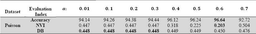
The accuracy percentage, NVI, and DB values for LINEX k-means clustering algorithms with different a in the simulated Poisson datasets.

We compute the skewness of them and run the k-means and the LINEX k-means algorithms with different values of a. The results are presented in Table 4. According to the results, it seems that the skewness affects the value of a, and in the skewed datasets, the accuracies of LINEX k-means algorithm with a > 0 are better than k-means algorithm. Therefore, we suggest scrutinizing how choosing the value of a depends on the skewness of the frequency curve of a dataset.

Table 4:

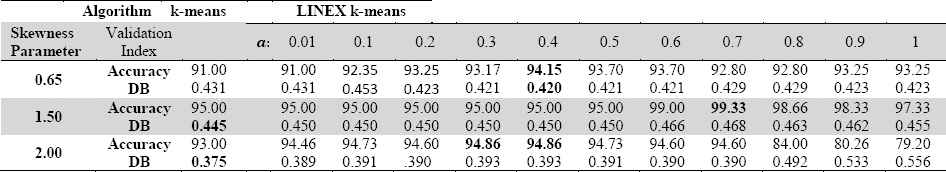
Evaluating the result of clustering three Exponential datasets with LINEX k-means and k-means algorithm. The first row for each skewness parameter is the accuracy percentages and the second row is the DB index.

5.2. Evaluation in some real datasets

Here we compare the results of LINEX k-means with k-means and k-median algorithms on some real datasets. We run the algorithms 500 times and compute the average of accuracies due to a random selection of centers for each algorithm. These datasets are all available in the UC Irvine Machine Learning Repository [2]. All the data are labeled so that we can evaluate the algorithms. We normalize the data before running the algorithm. The results are summarized in Table 5.

a)
The Iris data set is a collection of 150-flower specimen each with four features and is divided into three clusters.
b)
The Wine dataset consists of 178 chemical specimens of wine with thirteen features that partitioned into three clusters.
c)
The Hepatitis dataset contains 155 specimens with 19 categorical and numeric features, which is partitioned into two clusters.

Table 5:

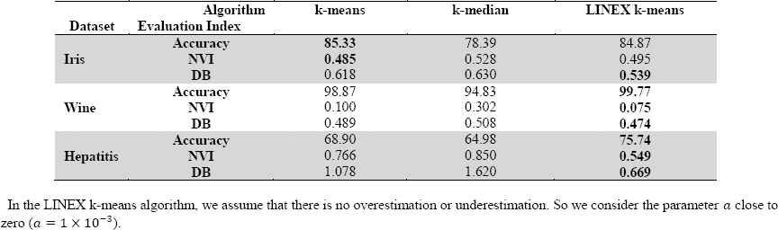
The accuracy percentage, NVI, and DB values for k-means, k-median, and LINEX k-means clustering algorithms in different datasets.

The results in Table 5 shows that LINEX k-means algorithm acts as well as the others and in some cases, it leads to better results. Normalizing the data improves the accuracy.

As we state before, sometimes the overestimating or underestimating is of different importance (For example, estimating the number of earthquakes with high magnitude during a short period in an Earthquake-prone area) and classifying an event in a specific cluster is worse (or better). Now consider three datasets: Seismic bumps, Haberman’s Survival and Magic Gamma Telescope.

d)
The seismic bumps dataset includes 2584 data with 18 categorical and numeric features, which describe the problem of forecasting high energy (higher than 104 J) seismic bumps in a coal mine and is partitioned into two clusters, “high energy seismic bump” and “no high energy seismic bumps”. Clustering a high-energy seismic bump as a no high-energy seismic bump is very hazardous.
e)
Haberman’s Survival includes 306 data with three integer features from a study on the survival of breast cancer patients who had tolerated surgery. It is partitioned into two groups, “the patient survived five years or more” and “the patient died less than five years”.
f)
Magic Gamma Telescope includes 19020 data with 11 real features, which use to describe high-energy gamma particles with the imaging technique in a ground-based atmospheric Cherenkov Gamma Telescope (The evidence of energy depositions is usually asymmetric along the major axis.). It is partitioned into two clusters, single and background. Classifying a background event as a signal is worse than clustering a signal event as the background. Therefore, the simple k-means algorithm is not appropriate for this dataset.

We use k-means and LINEX k-means algorithm with different values of a (as explained in the previous part) to partition data. We choose a according to the accuracy results and the NVI and DB values. The results in Table 6 shows that LINEX k-means algorithm is more accurate, especially when the overestimating and the underestimating are not of the same importance. The k-means and k-median algorithms that are based on symmetric dissimilarity distances are appropriate for data, which the negative and positive errors are of the same importance. However, the LINEX dissimilarity measure is useful in both symmetric and asymmetric cases.

Table 6:

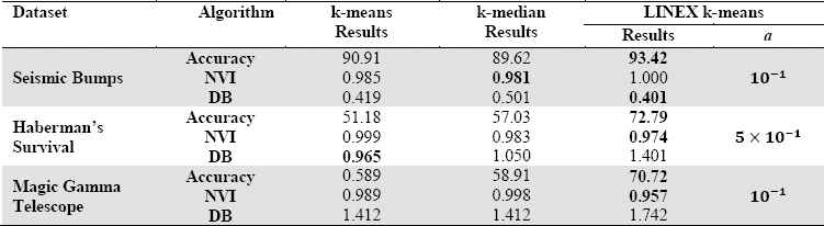
The accuracy percentage, NVI, and DB values for k-means, k-median, and LINEX k-means clustering algorithms in Seismic Bumps, Haberman’s Survival, and Magic Gamma Telescope datasets.

6. Conclusion

Sometimes we need an asymmetric dissimilarity measure to calculate the distance between data. We use the LINEX loss function as the dissimilarity measure in k-means clustering algorithm instead of the common measures such as squared Euclidean and Manhattan. So, the centers in each cluster are not the mean (or median) of their entities. To evaluate the accuracy of our algorithm, we partition some real and simulated datasets that their labels and their number of clusters are available and the NVI and the DB indexes help us both to compare the results and to choose a. In some of these datasets, the misclassifying the data into a special cluster may lead to a high loss. Therefore, it is important to use an asymmetric dissimilarity measure to make the different between overestimating and underestimating. Comparing the results, we conclude that LINEX k-means algorithm acts in almost cases well and partitioned the data accurately, especially when classifying an event in a specific cluster is worse (or better).

Acknowledgements

The authors would like to show gratitude to the editor and the reviewers of the article for their comments and suggestions on an earlier version of the manuscript which helped to improve the quality of content of the article.

References

[1]RC Amorim and P Komisarczuk, On Initializations for the Minkowski Weighted k-means, Lecture Notes in Computer Science, Vol. 7619, 2012, pp. 45-55.

[2]A Asuncion and DJ Newman, University of California, School of Information and Computer Science, Irvine, CA, 2007. UCI Machine Learning Repository http://www.ics.uci.edu/~mlearn/MLRepository.html]

[3]GH Ball and DJ Hall, A Clustering Technique for Summarizing Multivariate Data, Behavioral Science, Vol. 12, 1967, pp. 153-155.

[4]A Banerjee and S Merugu, Clustering with Bregman Divergences, Journal of Machine Learning Research, Vol. 6, 2005, pp. 1705-1749.

[5]L Bobrowski and JC Bezdek, C-means Clustering with the >LL1 and LL∞ Norms, IEEE Transactions on Systems, Man and Cybernetics, Vol. 21, 1991, pp. 545-554.

[6]PS Bradley, OL Mangasarian, and WN Street, Clustering via Concave Minimization, MC Mozer, M Jordan, and T Petsche (editors), Advances Neural Information Processing Systems, 1997, pp. 368-374.

[7]CWJ Granger, Outline of Forecast Theory Using Generalized Cost Functions, Spanish Economic Review, Vol. 1, 1999, pp. 161-173.

[8]M Halkidi, Y Batistakis, and M Vazirgiannis, Clustering Validity Checking Methods: Part II, ACM SIGMOD Record, Vol. 31, No. 3, 2002.

[9]TJ Harris, Optimal Controllers for Nonsymmetric and Nonquadratic Loss Functions, Technometrics, Vol. 34, 1992, pp. 298-306.

[10]JA Hartigan, Clustering Algorithms, Wiley, New York, 1975.

[11]Z Huang, Extensions to the k-means Algorithm for Clustering Large Data sets with Categorical Values, Data Mining and Knowledge Discovery, Vol. 2, 1998, pp. 283-304.

[12]AK Jain and RC Dubes, Algorithms for Clustering Data, Prentice-Hall, New York, 1988. reference series,

[13]K Kummamuru, R Krishnapuram, and R Agrawal, On Learning Asymmetric Dissimilarity Measures, ICDM ’05 Proceedings of the Fifth IEEE International Conference on Data Mining, 2005, pp. 697-700.

[14]DS Modha and WS Spangler, Feature Weighting in k-means Clustering, Machine Learning, Vol. 52, 2003, pp. 217-237.

[15]A Parsian and SNUA Kirmani, Estimation under LINEX Loss Function, Handbook of Applied Econometrics and Statistical Inference, Vol. 165, 2002, pp. 53-76.

[16]R Reichart and A Rappoport, The NVI clustering evaluation measure, In proceedings of the Thirteenth Conference on Computational Natural Language Learning, 2009, pp. 165-173.

[17]S Selim and M Ismail, K-means-type Algorithms: A Generalized Convergence Theorem and Characterization of Local Optimality, IEEE Transactions on Pattern Analysis and Machine Intelligence, Vol. 6, 1984, pp. 81-87.

[18]J Shao, Mathematical Statistics, second edition, Springer, 2003.

[19]HR Varian, A Bayesian Approach to Real Estate Assessment, SE Fienberg and A Zellner (editors), Studies in Bayesian Econometrics and Statistics in Honor of Leonard J. Savage, 1975, pp. 195-208.

[20]A Zellner, Bayesian Estimation and Prediction Using Asymmetric Loss Functions, Journal of the American Statistical Association, Vol. 81, 1986, pp. 446-451.

<Previous Article In Issue

Download article (PDF)

Next Article In Issue>

Journal: Journal of Statistical Theory and Applications
Volume-Issue: 17 - 1
Pages: 29 - 38
Publication Date: 2018/03/31
ISSN (Online): 2214-1766
ISSN (Print): 1538-7887
DOI: 10.2991/jsta.2018.17.1.3 How to use a DOI?
Open Access: This is an open access article under the CC BY-NC license (http://creativecommons.org/licences/by-nc/4.0/).

Cite this article

ris enw bib

TY  - JOUR
AU  - Narges Ahmadzadehgoli
AU  - Adel Mohammadpour
AU  - Mohammad Hassan Behzadi
PY  - 2018
DA  - 2018/03/31
TI  - LINEX K-Means: Clustering by an Asymmetric Dissimilarity Measure
JO  - Journal of Statistical Theory and Applications
SP  - 29
EP  - 38
VL  - 17
IS  - 1
SN  - 2214-1766
UR  - https://doi.org/10.2991/jsta.2018.17.1.3
DO  - 10.2991/jsta.2018.17.1.3
ID  - Ahmadzadehgoli2018
ER  -

download .riscopy to clipboard