
A note on Sum, Difference, Product and Ratio of Kumaraswamy Random Variables
- DOI
- 10.2991/jsta.2018.17.2.4How to use a DOI?
- Keywords
- Ratio of random variables; product of random variables; Kumaraswamy distribution; sub-independence
- Abstract
Explicit expressions for the densities of S = X1 + X2 , D = X1 − X2 , P = X1X2 and R = X1/X2 are derived when X1 and X2 are independent or sub-independent Kumaraswamy random variables. The expressions appear to involve the incomplete gamma functions. Some possible real life scenarios are mentioned in which such quantities might be of interest.
- Copyright
- Copyright © 2018, the Authors. Published by Atlantis Press.
- Open Access
- This is an open access article under the CC BY-NC license (http://creativecommons.org/licences/by-nc/4.0/).
1. Introduction
Kumaraswamy (1980) [3] introduced a two parameter absolutely continuous distribution which compares extremely favorably, in terms of simplicity, with the beta distribution. The Kumaraswamy distribution on the interval (0,1), has its probability density function (pdf) with two shape parameters a > 0 and b > 0 defined by
If a random variable X has pdf given in (1.1) then we will write X ∼ K(a,b).
The density function in (1.1) has similar properties to those of the beta distribution but has some advantages in terms of tractability. The Kumaraswamy pdf is unimodal, uniantimodal, increasing, decreasing or constant depending (similar to the beta distribution) on the values of the parameters. It has some basic properties of the beta distribution: a > 1 and b > 1 (unimodal); a < 1 and b < 1 (uniantimodal); a > 1 and b ≤ 1 (increasing); a ≤ 1 and b > 1 (decreasing); a = b = 1 (constant). For a detailed survey of properties of the Kumaraswamy distribution, the reader is referred to Jones (2009) [2]. This distribution has a close relation with beta and generalized beta (first kind) as listed below:
- •
If X ∼ Beta(1,b) then X ∼ K(1,b)
- •
If X ∼ Beta(a,1) then X ∼ K(a,1)
- •
If X ∼ K(a,b), then X ∼ GB1(a,1,1,b),
In this article we consider two independent (or sub-independent) Kumaraswamy random variables with appropriate parameters and study the convolution of their distributions (i.e., sum, difference, product and ratio). Also, we discuss some real life scenarios in which such convolutions might be an attractive model. This is the major contribution of this article. We list in sequel, the scenarios where sums, differences, products and ratios of two independent Kumaraswamy might be useful.
- •
Situations in which Kumaraswamy sums will be useful:
- —
Length or weight of a chain with n links.
- —
Electric resistance of a series circuit.
- —
The total life length of n products, where the next one is put on operation after failure of the preceding one.
In each of these cases, individual items (for example Xi denoting individual links for the first example, individual resistance for the second example and individual life length for the third example) can be considered as having univariate Kumaraswamy densities.
- —
- •
Situations in which Kumaraswamy differences will be useful:
- —
Let us suppose that in a certain mass-produced assembly, a 5 cm shaft must slide into a cylindrical sleeve. Shafts are manufactured whose diameter X1 follows a Kumaraswamy distribution and cylindrical sleeves are manufactured whose internal diameter X2 follows another Kumaraswamy distribution. Assembly is performed by selecting a shaft and a cylindrical sleeve at random. Suppose our interest is the following: In what proportion of cases will it be impossible to fit the selected shaft and cylindrical sleeve together. Clearly, the shaft and cylindrical sleeve will fit together only if the diameter of the shaft is smaller than the internal diameter of the cylindrical sleeve. We need the difference of the two random variables X2 and X1 to be greater than zero. We can take the difference X2 − X1 and find its distribution.
- —
- •
Situations in which Kumaraswamy product will be useful:
We cite a real life application below:
- —
An observer’s information about a classical system is captured by the observation that he/she assigns to it. It is a legitimate assumption that the two observers do not have to have the same information about the classical system. Next, if two observers have obtained their information about the system independently, then clearly together they have gathered more information about the system than each has individually. A natural question then is: is it possible to come up with a single observation which embodies their combined information? An answer to this question may be provided by considering distribution of the product of the two independent random variables.
- *
In evaluating the revenue from holding an asset defined by initial investment (X1) × net return(X2).
- *
Consider the portfolio value accumulation scenario: A portfolio with current value X1 will become X1 (1 + X2) after some period, here X2 is the interest rate and X1 and X2 are independent.
- *
ARCH models in time series studies.
- *
Number of cancer cells in tumor biology.
- *
- —
We believe that the above list of real life scenarios merits for the study of the distribution of the ratio
The rest of the paper is organized as follows: In Section 1, we discuss the distribution of the sum, difference, product and the ratio. Section 2 deals with the distribution (as in Section 1) under non standard Kumaraswamy univariate distributions. In Section 3, we present some ideas of constructing bivariate Kumaraswamy distribution via copula and possible extension to the multivariate case. In Section 4, some concluding remarks are provided.
For the derivation of the distributions of the sum S = X1 + X2, and of the difference D = X1 − X2, the assumption of independence is not needed, a much weaker concept called sub-independence (defined below) can replace that of independence.
For the sake of completeness we will state below a few definitions related to the concept of sub-independence. The concept of sub-independence is stated as follows: The rv ’s (random variables) X and Y with cd f ’s FX and FY are s.i. (sub-independent) if the cd f of X + Y is given by
The equations (1.3) and (1.4) above are in terms of cd f and c f . The definition of sub-independence in terms of events, similar to that of independence, is as follows.
We observe that the half-plane H = {(x,y) : x + y < 0}(⊆ ℝ2) can be written as a countable disjoint union of rectangles:
Definition 1.1.
The continuous rv ’s X and Y are s.i. if for every c ∈ ℝ
Remark 1.1.
- (a)
The representation (1.4) can be extended to the multivariate case as well.
- (b)
For a detailed treatment of the concept of sub-independence, please refer to Hamedani(2013) [1].
Consider the distribution of the sum S = X1 + X2 when the rv’s X1 and X2 are s.i., then pd f of S is the convolution of the pd f ’s of X1 and X2, which is given by
The distribution of the difference D = X1 − X2 when the rv’s X1 and −X2 are s.i., has a pd f which is the convolution of the pd f’s of X1 and −X2, given by
Now, assuming that the rv’s X1 and X2 are independent, then pd f ’s of P = X1 X2 and of
2. Kumaraswamy Sums, Differences, Products and Ratios
In this section we consider explicit expressions for the pdfs of S, D, P and R respectively. Note that for S and D, we employ the concept of sub-independence.
2.1. Explicit expression for the pdf of the Sum (S)
Theorem 2.1.
For 0 < s < 2, the pdf of S will be
Proof.
Consider the case 0 < s < 1, we have from (1.6),
The result for 1 < s < 2 can be established similarly. Hence the proof.
Some representative density plots for S is provided in Figures 1 and 2. The following observations can be made from these two graphs.
- •
When b1 and b2 are kept fixed, if all other possible combinations of the first two shape parameters (i.e., a1 and a2), the density appears to be slightly left-skewed (except for the case a1 = a2, in which it is approximately symmetric, as expected) (see Figure 1).
- •
When a1 and a2 are kept fixed, if all other possible combinations of the second two shape parameters (i.e., b1 and b2), the density appears to be slightly right-skewed (except for the case b1 = b2, in which it is approximately symmetric, as expected) (see Figure 2).

Density plot of S with b1,b2 fixed.

Density plot of S with a1,a2 fixed.
As a consequence, in order to model bounded risks (with a proper modification, if required, to be in the interval [0,1]) with a right skewed data, one might consider the scenario of changing the second shape parameter and keeping the first shape parameter fixed and vice versa for the left skewed data.
2.2. Explicit expression for the pdf of the Difference (D)
Theorem 2.2.
For −1 < d < 1, the pdf of D will be
Proof.
Similar to that of Theorem 2.1.
Some representative density plots of D are provided in Figures 3 and 4. The following observations can be made from these two graphs.
- •
When b1 and b2 are kept fixed, the density appears to be slightly right skewed, if a1 < a2 and left-skewed if a1 > a2, with the obvious symmetric scenario is which a1 = a2 (see Figure 3).
- •
When a1 and a2 are kept fixed, the density appears to be slightly left -skewed, if b1 < b2. Noticeably, the density appears to be approximately symmetric in the remaining two parametric configurations (i.e., in b1 = b2 and b1 > b2) (see Figure 4).
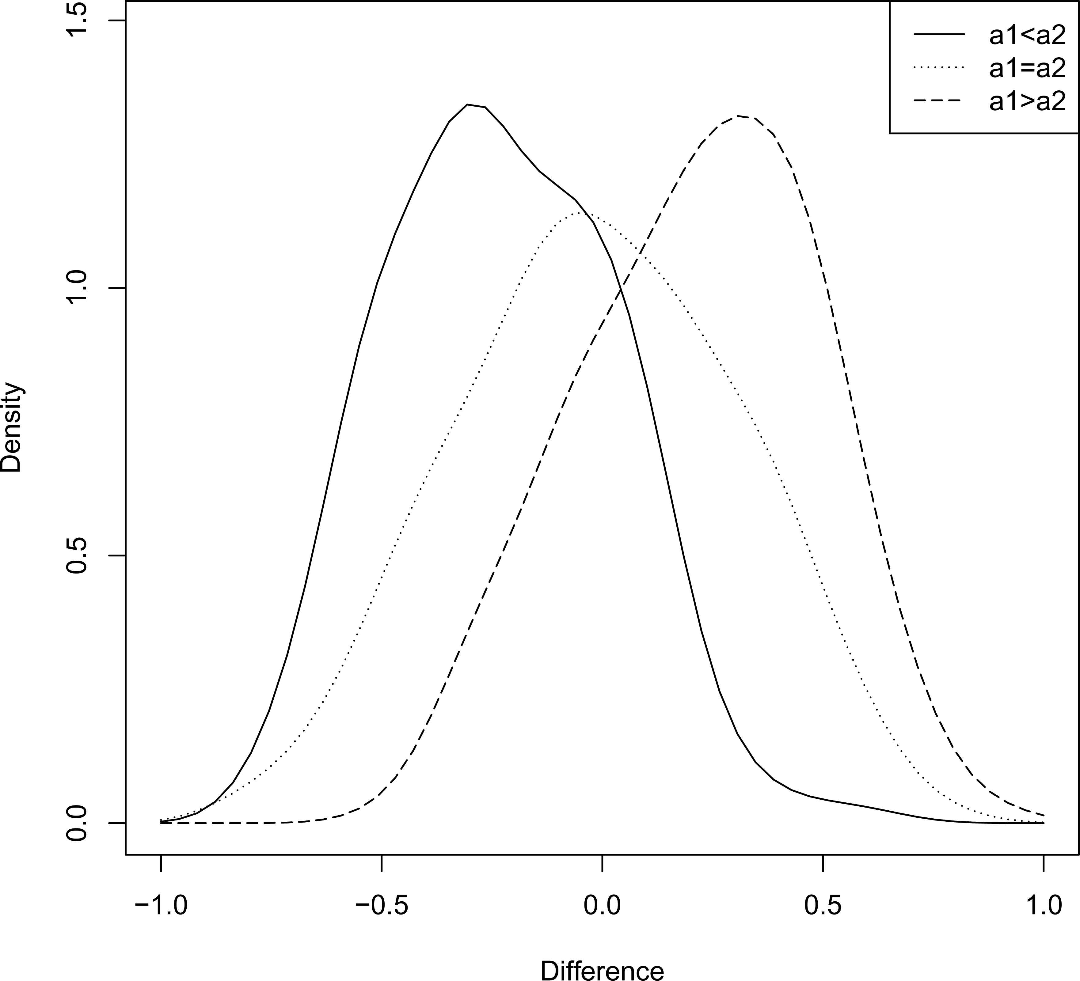
Density plot of D with b1,b2 fixed.
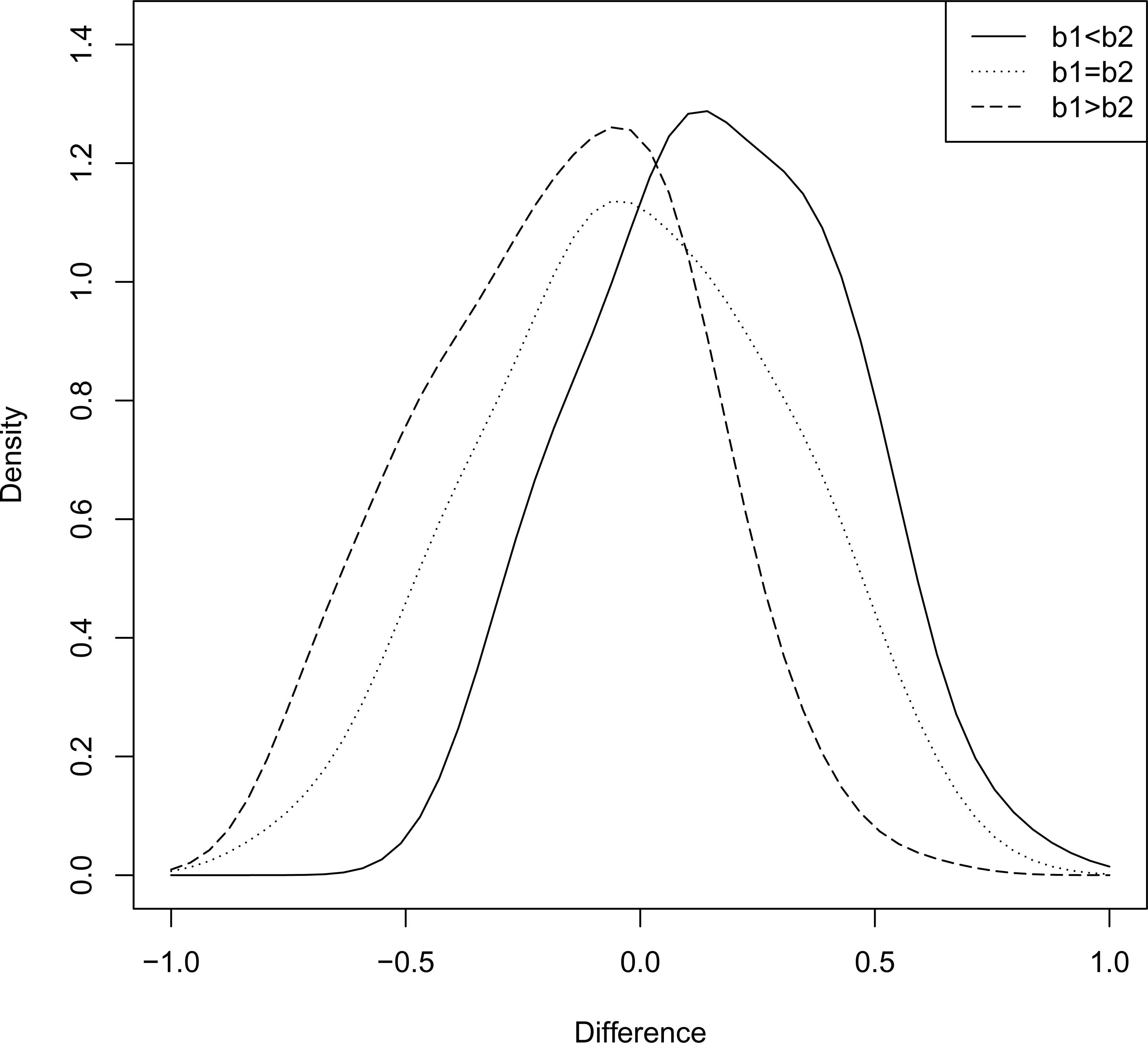
Density plot of D with a1,a2 fixed.
It appears that for the difference, the form of the density is very sensitive to any change in the first shape parameters (i.e., a1 and a2).
2.3. Explicit expression for the pdf of the Product (P)
Theorem 2.3.
For 0 < p < 1, the pdf of P will be
Proof.
From (1.8), we can write
Hence the result.
Some representative density plots of P are provided in Figures 5 and 6. From both of these plots it appears that regardless of the choice of the for four shape parameters, the density of P is right skewed.
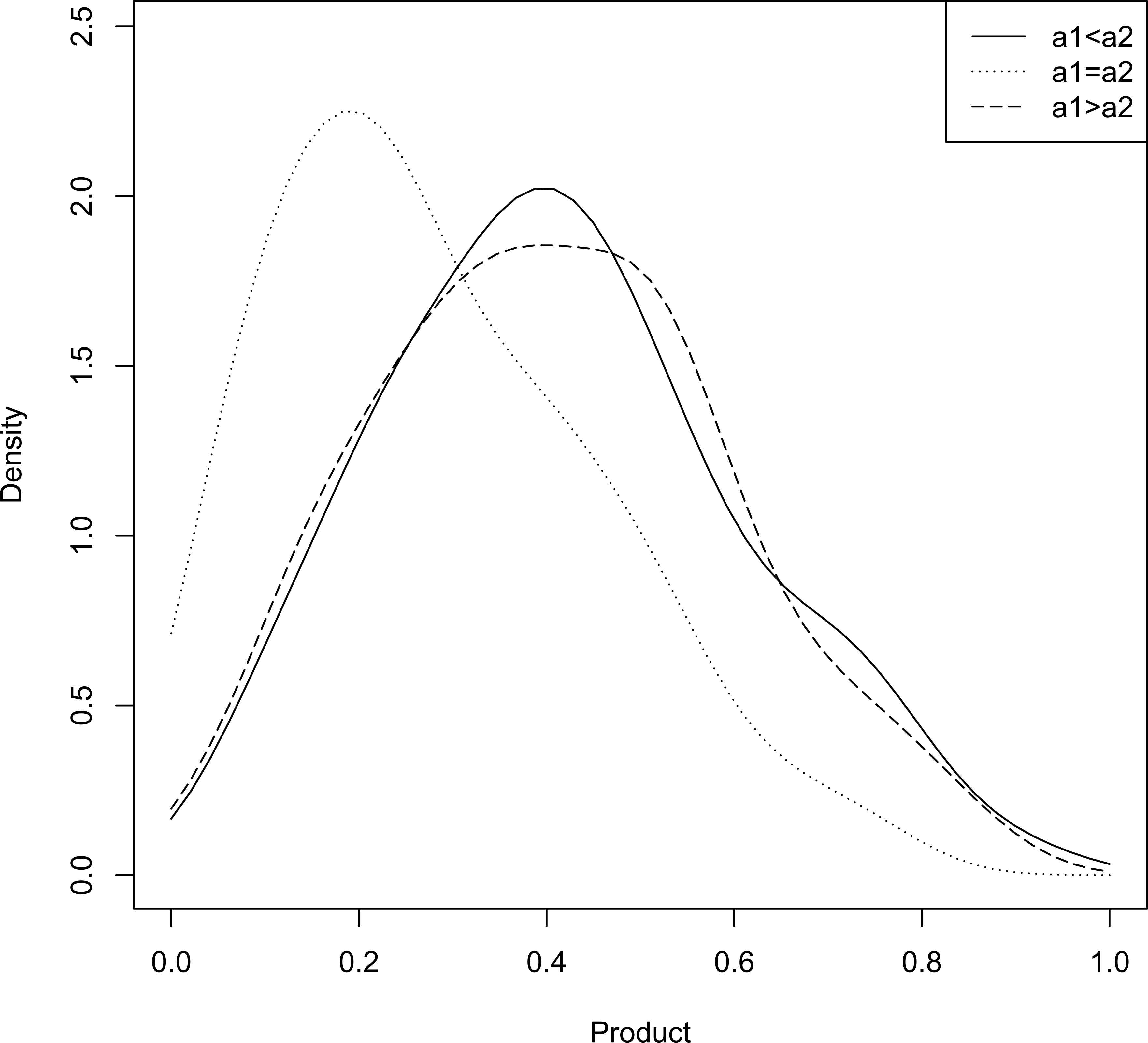
Density plot of P with b1,b2 fixed.
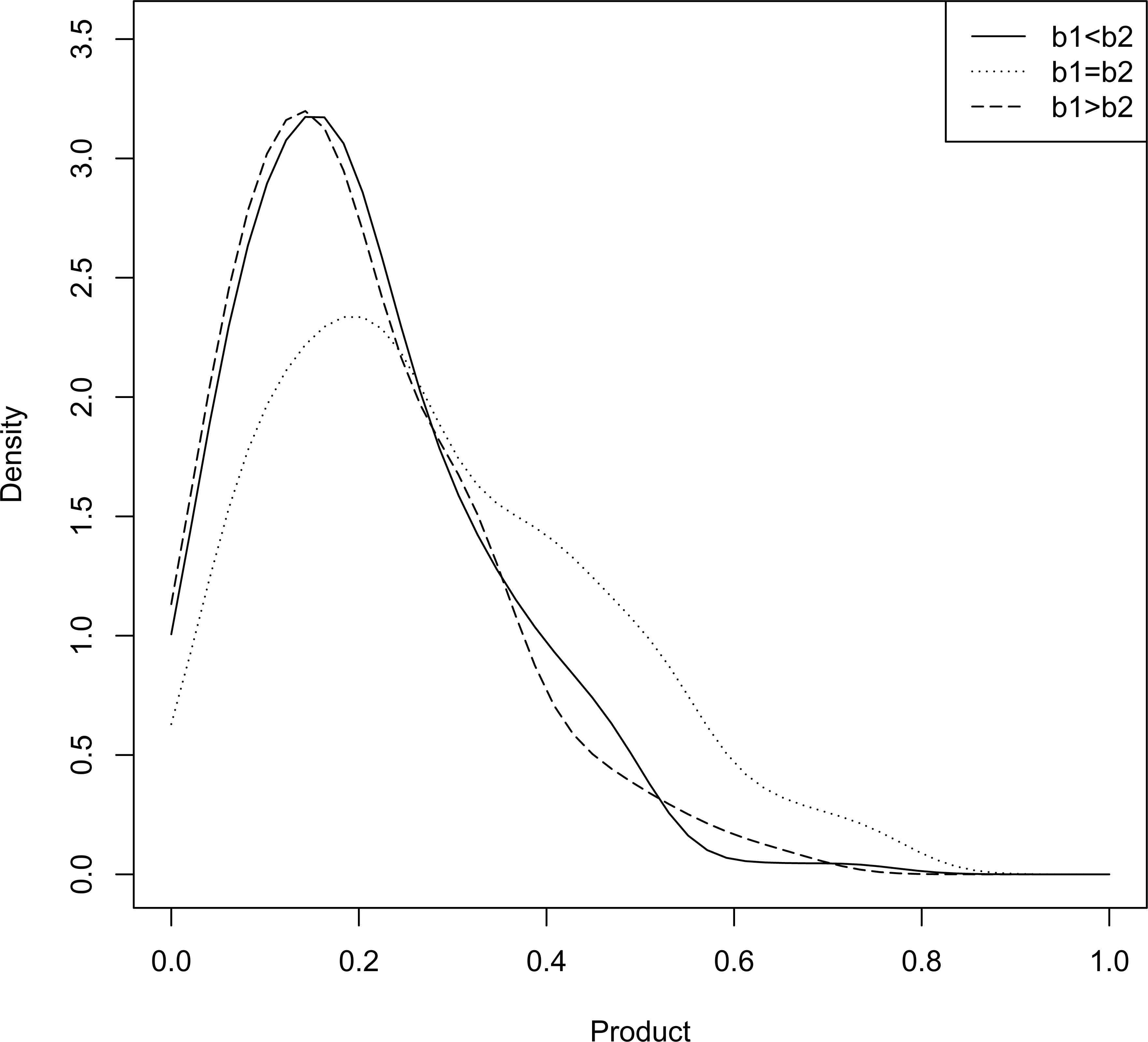
Density plot of P with a1,a2 fixed.
2.4. Explicit expression for the pdf of the Ratio (R)
Theorem 2.4.
For 0 < r < ∞, the pdf of R will be
Proof.
Let us consider the case 0 < r ≤ 1. From (1.9), we can write
The result for 1 < r < ∞ can be established similarly. Hence the proof.
Note: If b2 − 1 is an integer, the sum will stop at b2 − 1.
Some representative density plots of R are provided in Figures 7 and 8. From both these plots it appears that regardless of the choice of the for four shape parameters, the density of R is strictly right skewed.
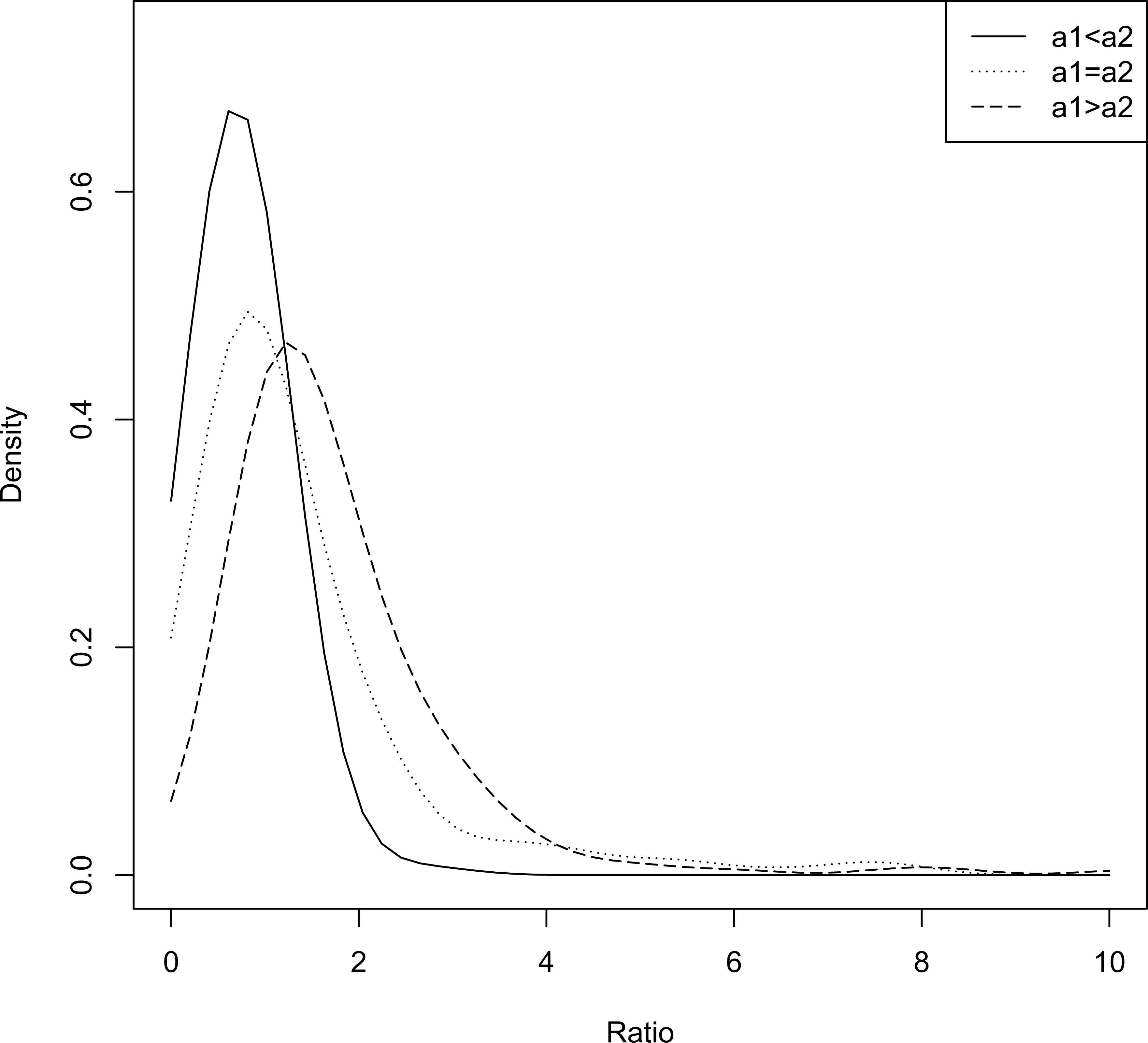
Density plot of R with b1,b2 fixed.

Density plot of R with a1,a2 fixed.
Remark 2.1.
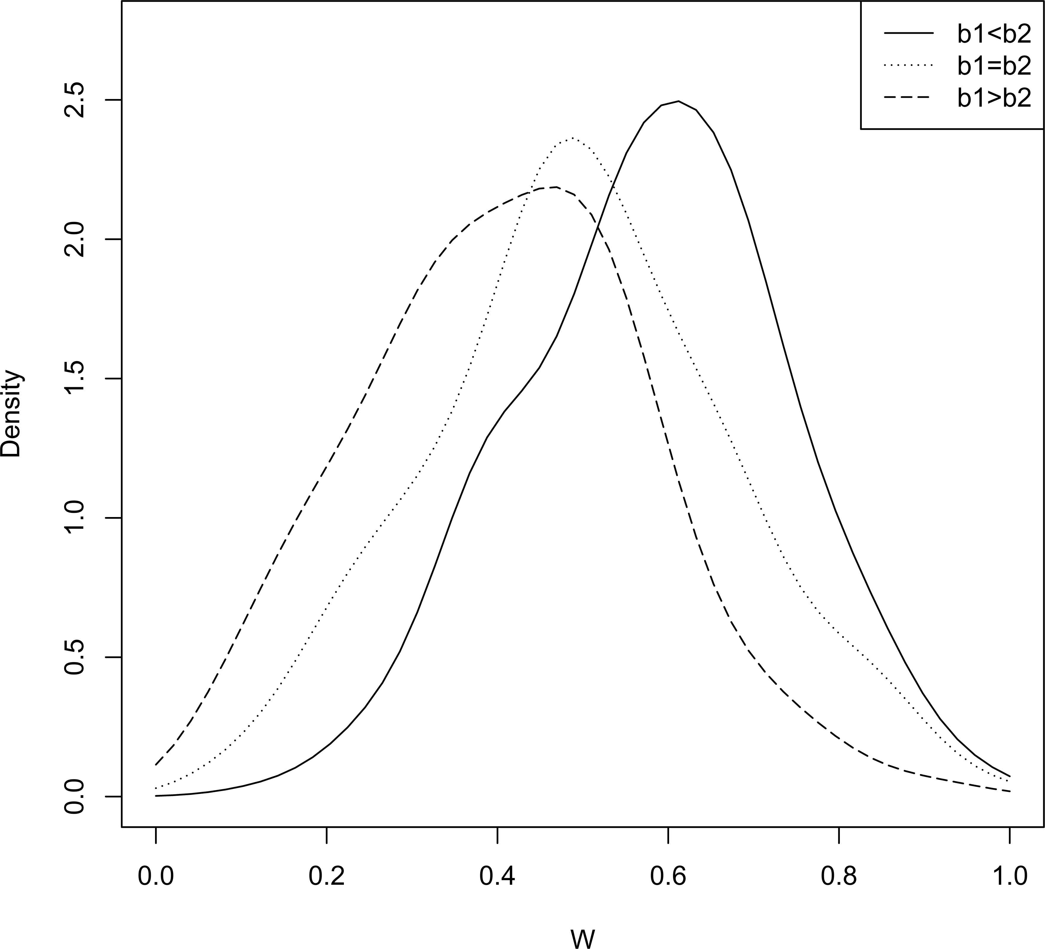
We have also provided some representative density plots (see Figures 9 and 10) for the density of
Density plot of W with b1,b2 fixed. Density plot of W with a1,a2 fixed.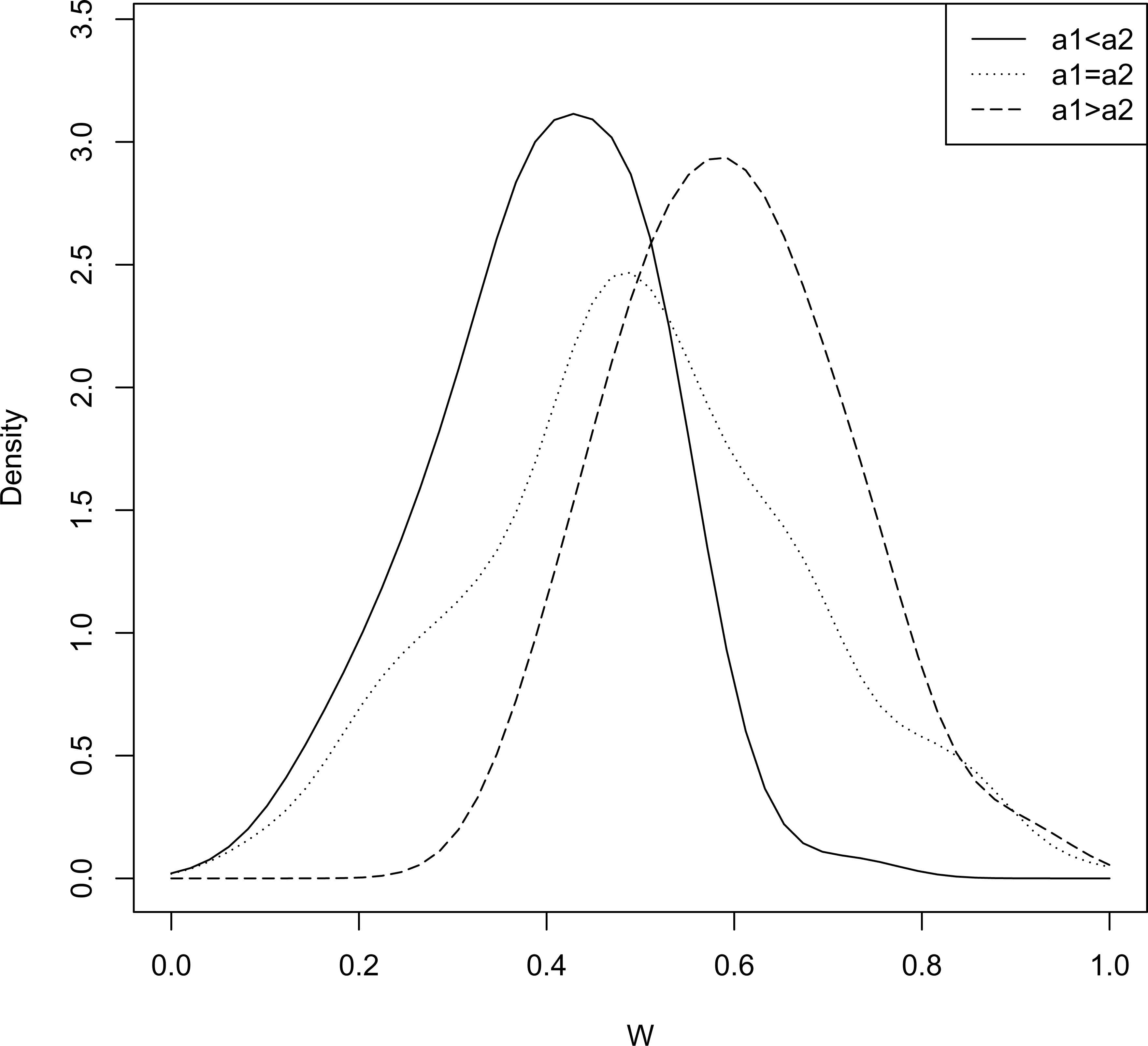
3. Sum, Difference, Product and Ratio for non-central Kumaraswamy distribution
In this section we will make frequent use of the following representation of a Kumaraswamy variable as a power of a Beta variable. If Y ∼ Beta(1,b), then X = Y1/a ∼ K(a,b). Next, we start with three non-central beta models (for details, see Nagar et al. (2013) [4]) and subsequently obtain the expression of the densities of Sum (S) , Product (P) and the Ratio (R).
The non-central Type I beta distribution is given by
The Type I beta distribution is well known in Bayesian methodology as a prior distribution on the success probability of a binomial distribution. Next, setting a = 1 and then by making the transformation X = U1/α, (for any α > 0), the corresponding non-central Kumaraswmy (Type I) will be
For notational simplicity, henceforth we call the above distribution as X ∼ NCKW(TypeI)(α,δ,b). Next, we have the following theorem:
Theorem 3.1.
Suppose X1 ∼ NCKW(TypeI)(α1,δ1,b1) and X1 ∼ NCKW(TypeI)(α2,δ2,b2) and they are sub-independent. Then for 0 < s < 2, the pdf of S will be
Proof.
Similar to that of Theorem 2.1.
Theorem 3.2.
For −1 < d < 1, the pdf of D will be
Proof.
Similar to that of Theorem 2.2.
Theorem 3.3.
For 0 < p < 1, the pdf of P will be
Theorem 3.4.
For 0 < r < ∞, the pdf of R will be
Remark 3.1.
One can also obtain in a similar fashion, the distribution of the Sum, Difference, Product, Ratios from the following two other non-central Kumaraswamy distributions:
- •
Non central Kumaraswamy (Type II) given by
- •
Non central Kumaraswamy (Type III) given by
4. Conclusion
In this article, by using the traditional method of transformation of variables, we have obtained probability density functions of sum, difference, product of two independent random variables both having regular Kumaraswamy and also non-central Kumaraswamy (Type I) distribution. Furthermore, in recent times, the construction of bivariate and multivariate Kumaraswamy distributions has received a significant amount of attention. Possible future works that can be done based on this article are as follows:
- •
Possible applications of independent Kumarswamy sums, products and ratios.
- •
Construction of Kumaraswamy sums, products etc. via dependent set up.
- •
A comparison study between beta distribution Sums, Products, Ratios and Differences etc.
Future efforts will be made to address these points and subsequently be reported elsewhere.
References
Cite this article
TY  - JOUR
AU  - Avishek Mallick
AU  - Indranil Ghosh
AU  - G. G. Hamedani
PY  - 2018
DA  - 2018/06/30
TI  - A note on Sum, Difference, Product and Ratio of Kumaraswamy Random Variables
JO  - Journal of Statistical Theory and Applications
SP  - 230
EP  - 241
VL  - 17
IS  - 2
SN  - 2214-1766
UR  - https://doi.org/10.2991/jsta.2018.17.2.4
DO  - 10.2991/jsta.2018.17.2.4
ID  - Mallick2018
ER  -