
Effect of angulation and Reynolds number on recirculation at the abdominal aorta-renal artery junction
- DOI
- 10.1016/j.artres.2017.11.007How to use a DOI?
- Keywords
- Abdominal aorta; Atherosclerosis; Recirculation; Renal artery; Yeleswarapu model
- Abstract
We investigate the effect of renal artery angle variation and Reynolds number on the probability of formation of atherosclerosis-prone regions at the abdominal aorta-renal artery junction. The rheologically accurate shear-thinning Yeleswarapu model for blood is used to simulate flow in a 3-Dimensional T-junction whose dimensions are those of the human abdominal aorta-renal artery junction. The recirculation length and wall shear stresses are evaluated at the junction for steady, laminar flow using ANSYS FLUENT v14.5. The recirculation length and wall shear stresses are calculated for Reynolds number of 500–1500, and the angle of renal artery (with the horizontal axis) of −20° to +20°. Computational fluid dynamics analysis for the flow conditions used in present study show that the flow recirculation and low wall shear stress regions overlap at the top surface of renal artery downstream of the entrance and at the curved surface of abdominal aorta downstream of the junction, making these regions susceptible to atherosclerosis. Further investigations show that positive angles of renal artery have larger area of recirculation and larger low wall shear stress regions. The recirculation length increases with Reynolds number, and it is maximum when θ = +20°, and minimum when θ = −20°.
- Copyright
- © 2017 Association for Research into Arterial Structure and Physiology. Published by Elsevier B.V. All rights reserved.
- Open Access
- This is an open access article distributed under the CC BY-NC license.
Introduction
Blood is a bodily fluid which plays an important role in the functioning of the human body. Blood flows through complex formations like curvatures, bifurcations, and branches in the network of blood vessels, especially the coronary, abdominal, carotid and femoral vasculature.1 At these formations the flow is non-axial, and the wall shear stress is low, leading, over time, to formation of atherosclerotic lesions due to deposition of fatty matter. Each formation has its own geometric peculiarities, and hence merit reporting of the flow features individually in a computational study. We select the abdominal aorta-renal artery junction for consideration in this study. This formation is very important since atherosclerotic disease, when it affects the renal arteries, can result in renovascular hypertension and ischemic nephropathy.2 This is because the deposition of fatty matter (plaque) reduces the lumen area of the renal artery, and the kidney responds by activating the renin-angiotensin system to increase the blood pressure.3
Due to the recent increase in demand for the use of non-invasive tools and cutting edge technologies in biomedical engineering, Computational Fluid Dynamics (CFD) has been accepted as a tool to analyze fluid flow in human anatomy. The formation of atherosclerotic lesions,4 thrombosis,5 and calculation of Fractional Flow Reserve (FFR)6 can each be predicted using CFD. In the context of atherosclerotic plaque, the combination of CFD and images from Computed Tomography (CT)/Magnetic Resonance Imaging (MRI) will give realistic, accurate hemodynamic values that will help in effective identification of plaque growth in complex formations. Blood flow has been simulated in bifurcations and junctions by assuming that it behaves as a Newtonian fluid.7,8 Specifically, many recent articles, which have studied the flow of Newtonian fluid in abdominal aorta-renal artery junction, predict the growth of atherosclerotic plaque in both laminar and turbulent flows.3,9,10 However, the Newtonian assumption is a simplification because blood is non-Newtonian: in specific, it exhibits shear-thinning,11 viscoelastic12 and thixotropic13 behavior. There are several references 4,14–16 that show the importance of, and major differences between, using a non-Newtonian model over a Newtonian model for blood. In this study we use a non-Newtonian model for blood: in particular, we use a shear-thinning model as a first step.
Generalized Newtonian models that capture the shear thinning behavior of blood have been applied to understand the flow mechanics in bifurcations: these include the Casson,17 the Power-law,18 and the Carreau-Yasuda model.19 The earliest 3-Dimensional (3-D) frame-invariant model for blood, which had a function specifically fitted to shear-thinning viscosity data of human blood over a range of 0.05 s−1 to 600 s−1, was the model described in Yeleswarapu et al.15 Henceforth, we refer to this model as the Yeleswarapu model. The shear-thinning Yeleswarapu model has been used in steady and pulsatile flow simulations in an axisymmetric cylindrical pipe,20 axisymmetric stenosed pipe,21 and stenosed 2-D channel.14 However, the full potential of the model can be achieved only in CFD simulations of flow in 3D reconstructions of arterial branches in the human vasculature. In this work, we do this and then detail the hemodynamic insights gained from the flow analysis.
The present work deals with the CFD analysis of steady flow of blood, modeled using the shear thinning Yeleswarapu model, in a 3-D T-junction with the same dimensions as those of the human abdominal aorta-renal artery junction. The following range of conditions are used: Reynolds number (Re) = 500–1500 (this range is chosen as the flow in undiseased renal artery is laminar, and Re typically varies between 400 and 110022), and variation of renal artery angle θ with respect to horizontal axis = −20° to +20°.23,24 The problem is formulated in Section Method: the flow geometry is described, the model is introduced, the balance equations that need to be solved are written, and the numerical scheme is also detailed. The validation for the UDF implemented in our numerical analysis is given in Section Validation of methods. The results and discussion are given in Section Results and Discussion, respectively. A brief summary and possible future extensions of this work are given in Section Conclusions.
Method
Geometry
A 3D symmetric T-junction geometry representing the intersection of the renal artery and the abdominal aorta is generated in ANSYS 14.5. The 2-Dimensional (2-D) cross-sectional view of the junction is given in Fig. 1, and this clearly indicates θ to be the angle between the renal artery and the horizontal x-axis. Here, the dimensions (diameters, but not lengths) and angles of the T-junction are those of the abdominal aorta-renal artery junction as taken from clinical references23–25. The lengths of the abdominal aorta section and renal artery sections are chosen such that their effect on the computed recirculation length is minimum.

2D representation of abdominal aorta-renal artery junction.
A preliminary test is done to determine the length of the renal artery for which predictions of the reattachment length vary within acceptable limits. The length of renal artery branch is varied in multiples of the main branch diameter (D) as 5D, 10D, 15D and simulations are carried out at Re = 1000, which is a typical number for this geometry. The relative percentage difference of reattachment length was 0.64% for change in length from 10D to 15D, and hence 10D is chosen for further simulations.
Governing equations
We simulate the steady flow of blood, and model blood as a shear thinning fluid as a first step to assess the effect of non-Newtonian behavior on hemodynamic predictions in 3D geometries. The governing equations for steady, laminar, isothermal flow which includes the effect of gravity are given below.
Continuity:
Momentum balance:
Cauchy stress tensor:
The shear rate is given as:
The parameter Λ = 14.81 s is the shear thinning index, η0 = 0.0736 Pa s is the asymptotic apparent viscosity as
Boundary conditions
At the inlet: A fully developed velocity profile of the shear thinning fluid is imposed. This profile is generated by solving the equations for steady flow in a pipe.
At outlet of abdominal aorta and renal artery: Outflow boundary condition is imposed such that the flow rate in the renal artery is 27.6% of inlet flow rate.26
At abdominal aorta and renal artery walls: No slip boundary condition is used; u = 0,v = 0,w = 0.
Meshing
A structured non uniform grid is generated in ICEM CFD, and adapted for solving the flow in abdominal aorta – renal artery junction. The grid consists of hexahedral elements, and is highly clustered near the regions of large gradients and coarser near the regions of low gradients. The critical region where many changes are expected is at the junction where the flow diversion takes place: therefore a very fine grid is selected in that region.
Numerical scheme
The numerical simulations are carried out using commercial software ANSYS FLUENT v14.5 that implements finite volume method. The three dimensional, pressure based solver for laminar flow is used. Constant density ρ = 1050 kg/m3 and shear thinning viscosity from Yeleswarapu model are used. Shear-thinning viscosity from Yeleswarapu model is coded by means of a User-Defined Function (UDF). SIMPLE scheme is used to solve pressure–velocity decoupled equations. UPWIND scheme of second order is used to discretize convective terms of momentum equation. Inbuilt parallel computation is used to solve the simulations faster and reduce the CPU time.
Grid independence
The grid independence analysis is done for increasing number of cells at Re = 1000. The number of cells is increased by varying the nodes along the axial, azimuthal and radial direction, keeping the minimum grid spacing (δ) = 0.002 cm at the vicinity of the junction and along the renal artery. The percentage relative error for 1.2 million cells (compared with 2.8 million cells) is 0.96% for recirculation length (the variable of interest), and, since the error is within the desired <1% limit, 1.2 million cells is used as optimized grid for further computations.
Validation of methods
Steady flow in a cylindrical pipe
The results in Yeleswarapu et al.15 have already shown that the Yeleswarapu model gives more accurate results, for the velocity profiles of blood, compared to Newtonian model. The User Defined Function (UDF) of the shear-thinning Yeleswarapu model is validated by comparing the centerline velocities of the simulations in ANSYS FLUENT with the model analytical values and experimental data for steady flow of porcine blood in a pipe reported in Yeleswarapu et al.15 Steady flow in a 1/4 inch diameter pipe is simulated with mean inlet velocities of 0.01592, 0.01945, and 0.02476 m/s as done in Yeleswarapu et al.15 The parameters of the shear-thinning model in Eq. (5) are selected to be those of porcine blood (η0 = 0.2 Pa s, η∞ = 0.0065 Pa s, Λ = 11.14 s). The fully developed centreline velocity from simulations is compared with the experimental and analytical values reported in Yeleswarapu et al.,15 and the percentage error of simulations vs predicted values is reported in Table 1. The relative error between the simulations and the values predicted by Yeleswarapu model in Yeleswarapu et al.15 varies between 0.3% and 8.6%, and it is even lesser for the Newtonian model as it varies between 0.3% and 2.6% (see Table 1). In addition, a blunt profile near the centre line axis is observed, similar to that predicted by the Yeleswarapu model, and this is seen in Fig. 2. These confirm that the UDF has been coded correctly, and that simulations in FLUENT give satisfactory results.
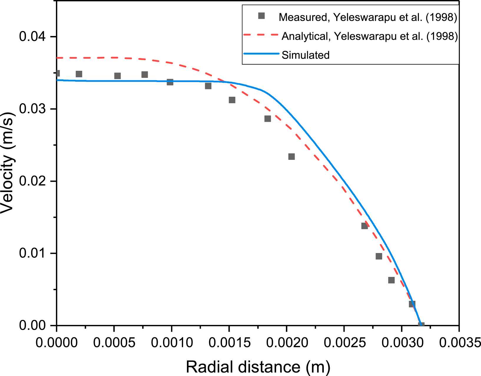
Velocity profile for measured, analytical and simulated values using shear thinning Yeleswarapu model of blood with mean inlet velocity of 0.02476 m/s.
| Mean velocity | Centerline velocity (experimental) | Centerline Velocity (Yeleswarapu model) | Centerline velocity (Newtonian model) | ||||
|---|---|---|---|---|---|---|---|
| Analytical | Simulated | % error | Analytical | Simulated | % error | ||
| 0.01592 | 0.0230 | 0.0232 | 0.0240 | 3.4 | 0.0318 | 0.0317 | 0.31 |
| 0.01945 | 0.0284 | 0.0287 | 0.0288 | 0.3 | 0.0390 | 0.0380 | 2.6 |
| 0.02476 | 0.0344 | 0.0370 | 0.0338 | 8.6 | 0.0496 | 0.0493 | 0.6 |
Validation of UDF in FLUENT. Comparison of mean velocities as obtained by simulations with the analytical values of Yeleswarapu model and experimental data. All values are in m/s.
Steady flow in T-junction
The UDF for shear thinning Yeleswarapu model is further validated by comparing results for blood flow in a T-junction (Fig. 3) with the results of Shibeshi and Collins16 for the same geometry. The axial velocities (at L1 and L2 in Fig. 3) and the wall shear stresses (at top and left wall) from the simulations for a steady flow in a T-junction are compared and found to give excellent fit with the data reported in Shibeshi and Collins16: this can be seen in Fig. 4(a–d). This confirms that the CFD simulation procedure we adopted (which incorporates the UDF) is able to predict the flow behavior accurately in both simple and complex geometries. These validations give us the confidence to analyze flow using the same tools in 3-D T-junction whose dimensions are similar to the human abdominal aorta-renal artery junctions.

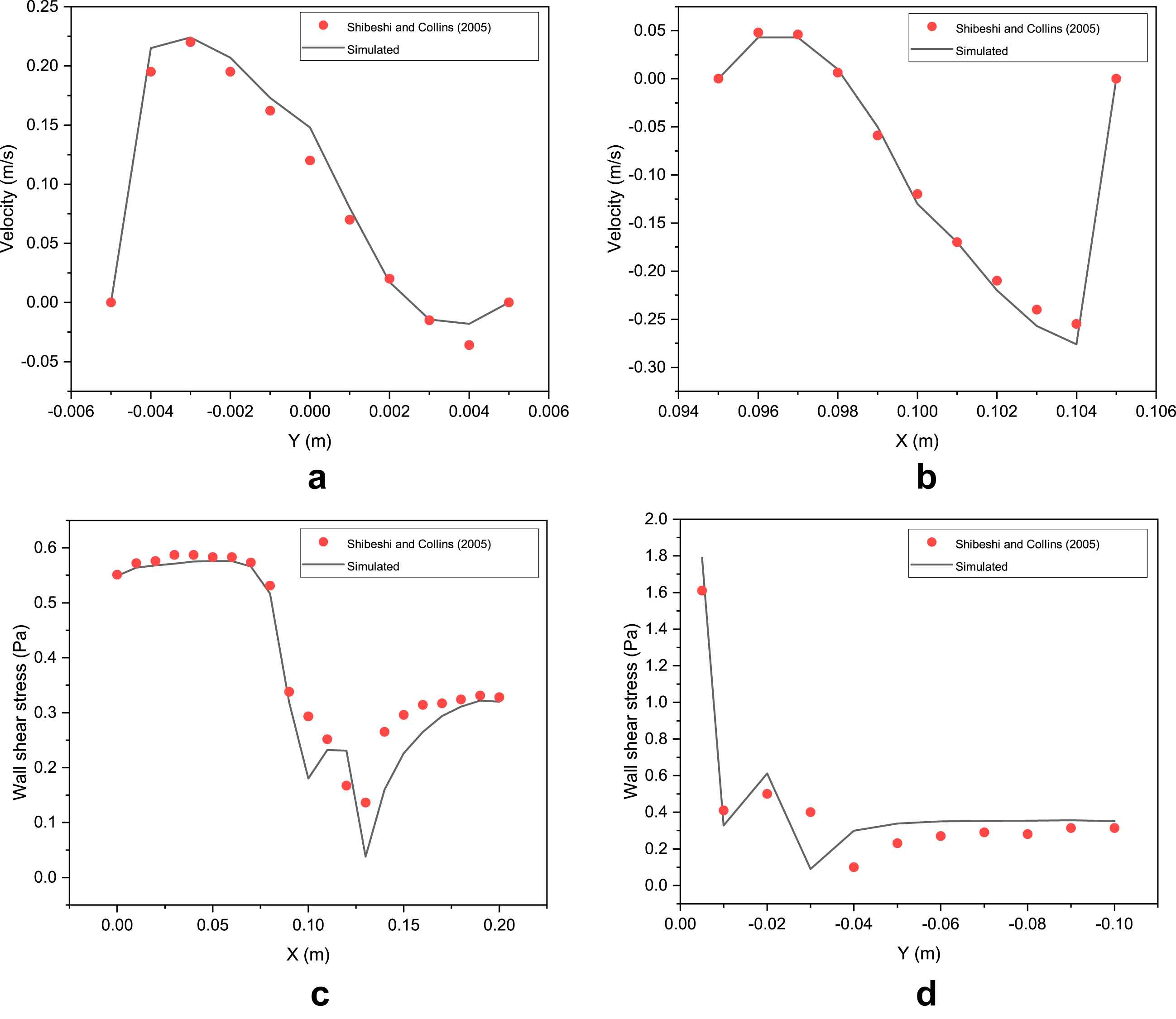
UDF validation for flow in a T-junction. Comparision of simulated values of (a)Axial velocity at L1, (b) Axial Velocity at L2, (c) Wall shear stress at top wall, and (d) Wall shear stress at left wall, with analytical data from Shibeshi and Collins.16.
Results
The flow characteristics in the abdominal aorta-renal artery junction depend on the diameters of abdominal aorta and renal artery, the Re and angle (θ) of renal artery with respect to the horizontal axis. The diameter of abdominal aorta is taken as 0.02 m and diameter of renal artery is taken as 0.005 m. The analysis demonstrates a strong relationship between the flow dynamics and the angulation of the renal artery.
Recirculation length versus Re
Figure 5 represents the flow pattern (recirculation) by way of streamlines in vicinity of the renal artery bifurcation for Re = 1000 at different angles. The results shows that recirculation region occurs at the upper surface of the renal artery, and downstream of the entrance where the renal artery branches out of the abdominal aorta. The region of recirculation when θ = +20° is large when compared to the recirculation area in θ = −20°. Figure 6 shows the streamlines at the symmetry plane in the main aorta branch. This recirculating flow pattern is observed in all the cases studied in the present work.
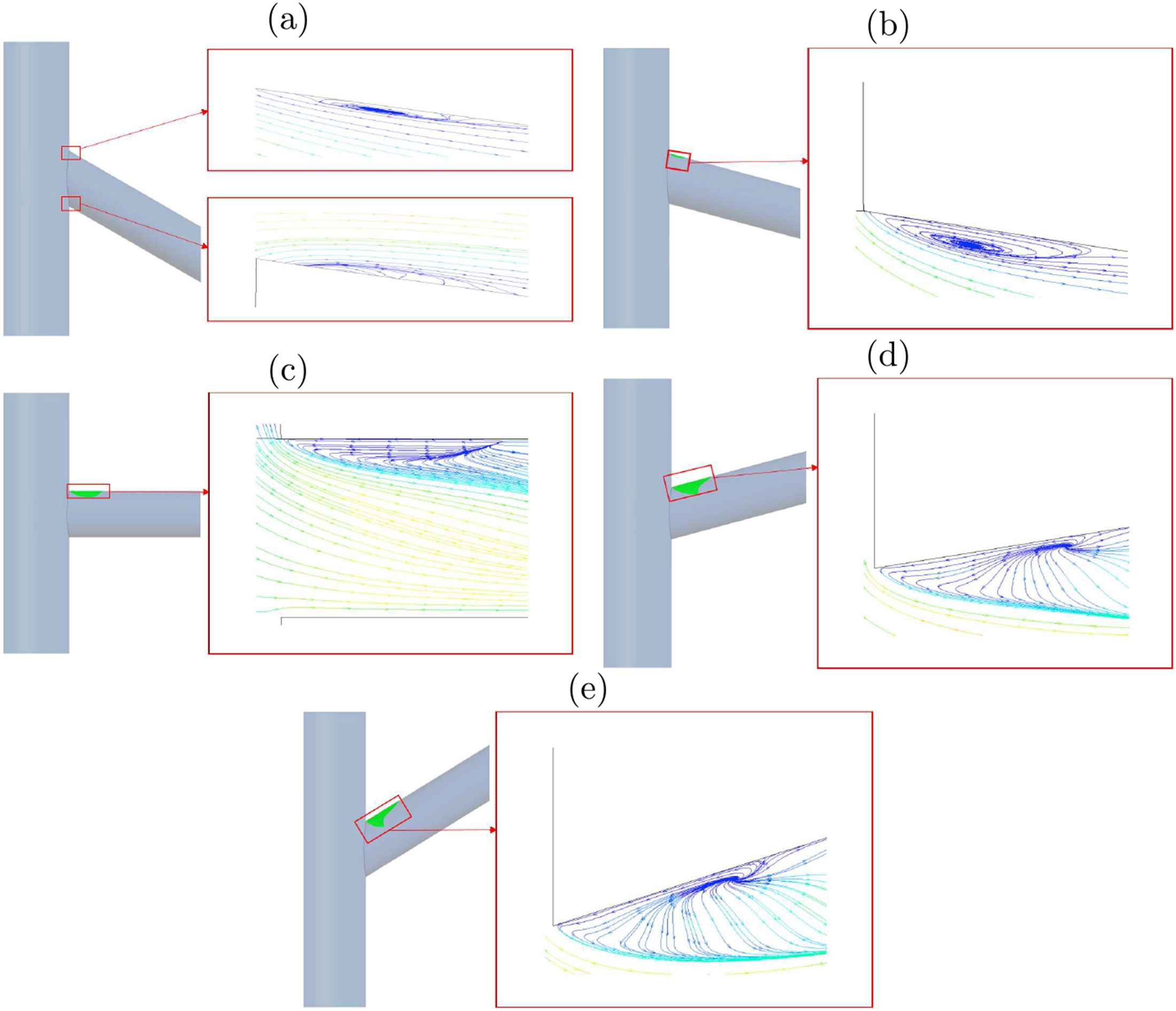
Regions of recirculation in renal artery with streamlines for Re = 1000 and (a) −20°, (b) −10°, (c) 0°, (d) +10°, (e) +20° of renal artery.
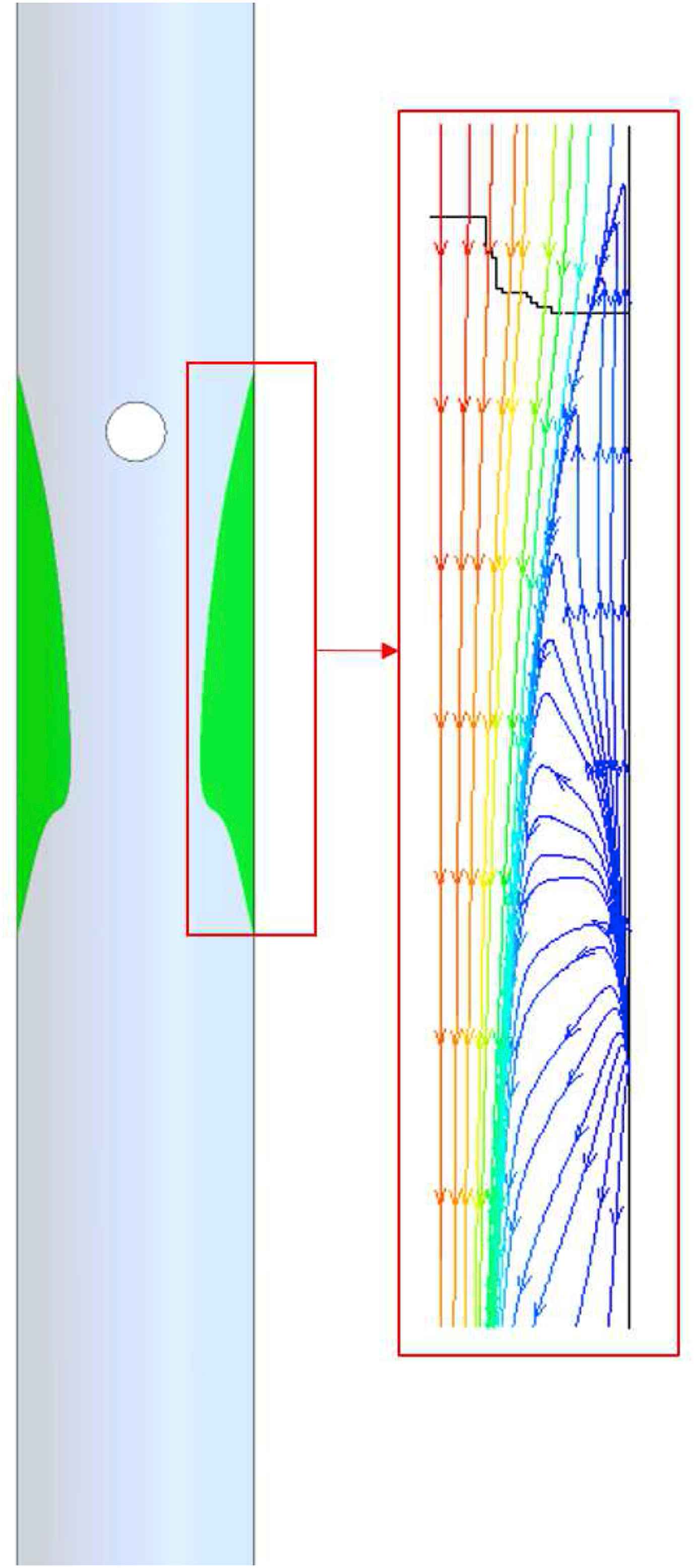
Recirculation region with streamlines in the abdominal aorta.
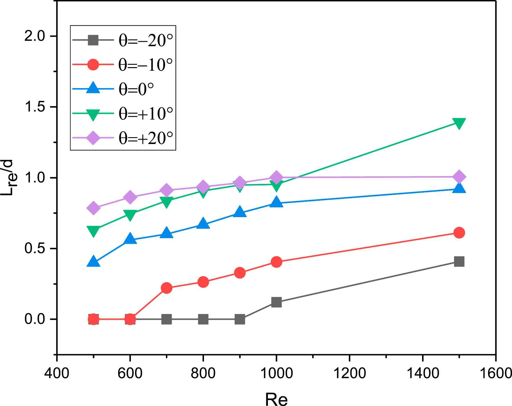
Recirculation length Vs Re at various angles of the renal artery.
The recirculation length is determined as the distance between the entrance and the point at the wall where the velocity vector changes sign. Figure 7 shows the variation of non-dimensional recirculation length for different Re and angular variation of the renal artery branch. Lre/d increases with increase in Re for a fixed θ, and decreases with decrease in θ for a fixed Re. The maximum Lre/d is when θ = +20°. For the given flow conditions, the recirculating regions is observed to occur in the renal artery at Re = 500 itself for θ = +20°, +10°, 0°, whereas it appears only at Re = 700 fo θ = −10° and at Re = 1000 for θ = −20°, respectively.
Wall shear stress variation in steady flow
Figure 8 shows the variation of wall shear stress as a contour in the abdominal - aorta renal artery junction for the different angular variations at Re = 1000. This analysis shows that the low WSS occurs on the upper surface of the renal artery downstream of entrance. The region of low wall shear stress overlaps with the region of recirculation. This confirms that these regions of the abdominal aorta-renal artery junction are most prone to atherosclerosis: this is a novel prediction of our study. Further, the extent of low wall shear stress region varies with the angle of renal artery. This confirms the dependence of atherosclerosis-prone region on angular variation as demonstrated in Fig. 7.

Variation of wall stress on the top surface of the renal artery for different angles.
Discussion
We used a CFD simulation procedure to identify regions prone to atherosclerosis in the 3D abdominal aorta-renal artery junction: we evaluated the hemodynamic forces and recirculation length for the physiologically relevant shear thinning model of blood. Prior to CFD simulations in actual geometry, the grid independence test and the model validation is necessary to ensure the results obtained are reliable and accurate. The simulation results for flow in a straight pipe shown in Table 1 compare well with the analytical solution obtained for the Yeleswarapu model, and are also very close to the experimental values of Yeleswarapu et al.15This confirms that the UDF is coded accurately. In addition, the simulation results of axial velocity profile (Fig. 4 (a) and (b)) and wall shear stress profile (Fig. 4 (c) and (d)) for steady flow in T-junction, give excellent match with the simulation results in Shibeshi and Collins.16 This confirms that the CFD simulation procedure is reliable and accurate in predicting the blood flow behavior through T-junction geometries.
Results from our CFD simulations in the abdominal aorta-renal artery junction predict low wall shear stress and large recirculation zones at the upper surface of the renal artery downstream of the entrance, and on the curved surface at the side of the abdominal aorta downstream of the junction. This indicates that atherosclerotic plaque is likely to form at these locations in the abdominal aorta-renal artery junction: this is a novel prediction of our study. Our predictions are consistent with earlier studies1,27 which show that specific locations such as branches and curvatures in arteries are susceptible for atherosclerosis. Further we included the effect of Re and renal angular variation on the local hemodynamics: we recorded that the size of the region prone to atherosclerotic plaque decreases with the decrease in angle of renal artery, but increases with increase in Re.
The length of recirculation determines the area of plaque deposition: larger the length of recirculation, more is the plaque formed to restrict the flow area. The decrease of recirculation length with decrease in θ as in Fig. 7 can be understood in the sense that, as the angle with the horizontal (θ) decreases, the flow in the renal artery is in the direction of main stream flow leading to earlier reattachment of the flow. Similarly, when θ increases, the flow in the renal artery is pulled away from the main stream flow leading to delayed reattachment. These CFD predictions are consistent with the results for the hemodynamics in coronary artery with angle variation,28 where the wides angles of coronary arteries had larger recirculation compared to the small angles variations. This match shows that the simulations are making reasonable predictions, and one may therefore proceed to evaluate their quantitative match with experimental data where available.
The wall shear stress regulates the behavior of the endothelial cell layer and influences the diffusion of macromecules into the artery walls.29 The region of low wall shear stress occurs where there is flow reversal and increases the probability of plaque in that region. Figure 8 shows that, the low wall shear stress region at the top surface of renal artery is larger for positive angles of renal artery, and maximum at θ = +20°. Also, for the given flow conditions, large regions of low wall shear stress and recirculation zone are collocated on the abdominal aorta downstream of the junction with the renal artery (observed but not shown), making it susceptible to atherosclerosis.
Conclusions
Assessment of hemodynamic conditions using CFD has great potential in non-invasive medical planning. In this study, CFD simulations are used to study the effects of renal artery angulation and Reynolds number on the hemodynamics of the abdominal aorta-renal artery junction. Our CFD findings show that the upper surface of the renal artery downstream of entrance, as well as the side curved surface of the abdominal aorta downstream of the junction, are prone to formation of atherosclerotic plaque. The recirculation length - an indicator of size of plaque - increases with Reynolds number, and increasing positive angulation. Low wall shear stress zone in the renal artery region is maximum when the angulation is a high positive value. The results provided here for non-invasive estimation of hemodynamic factors are found to be sound, and the method has potential for identifying geometries that are prone to renovascular diseases. The results need to be verified with clinical observations.
This work has limitations and requires further extension. The wall is considered to be rigid rather than elastic, therefore it does not fully resemble the physiological properties of a abdominal aorta-renal artery junction. Further work can include CFD simulation in patient derived geometries constructed from CT/MR. Also the simulation results were obtained under the assumption of steady flow conditions. Use of pulsatile flow conditions and obtaining the temporal hemodynamic indicators can be further extension of present work.30
Conflict of interest statement
The authors have no conflicts of interest to disclose.
Acknowledgement
M. Ameenuddin was supported by the
Appendix A
Supplementary data
Supplementary data related to this article can be found at
References
Cite this article
TY  - JOUR
AU  - Mohammed Ameenuddin
AU  - Mohan Anand
PY  - 2017
DA  - 2017/12/14
TI  - Effect of angulation and Reynolds number on recirculation at the abdominal aorta-renal artery junction
JO  - Artery Research
SP  - 1
EP  - 8
VL  - 21
IS  - C
SN  - 1876-4401
UR  - https://doi.org/10.1016/j.artres.2017.11.007
DO  - 10.1016/j.artres.2017.11.007
ID  - Ameenuddin2017
ER  -