
Detection of Land in Marine Images
Corresponding author. Email: t.praczyk@amw.gdynia.pl
- DOI
- 10.2991/ijcis.2018.125905640How to use a DOI?
- Keywords
- Horizon line detection; Land segmentation; Marine images
- Abstract
In order to navigate safely at sea, contemporary marine vehicles, both surface and underwater, are equipped with a variety of different sensors. One of these sensors is typically a video camera, a device that is becoming increasingly popular on the decks of both ships and smaller marine vehicles. A compact size and low cost make it an appealing sensor particularly for small and medium size autonomous vehicles which utilize the camera mainly for obstacle detection and collision avoidance. However, the visual information provided by the camera can also be combined with information acquired from the navigational map, for estimating the position of the vehicle in the environment. In this paper, an the coast can be estimated and then utilized to calculate vehicle position. The paper formulates the algorithm and reports verification experiments on real images of the Gdynia harbor and its neighborhood.
- Copyright
- © 2019 The Authors. Published by Atlantis Press SARL.
- Open Access
- This is an open access article distributed under the CC BY-NC 4.0 license (http://creativecommons.org/licenses/by-nc/4.0/).
1. INTRODUCTION
Marine navigation in coastal areas differs from that in the open sea. Due to the proximity of land it is necessary to take considerable measures to ensure safety. In order to maintain a safe distance from dangerous land objects, continuous monitoring of the external world with the use of all available systems, devices, and sensors is advisable. To this end, navigational radar is typically used when possible, however, it is generally only available on merchant vessels, navy ships, fishing boats, and larger yachts. Small marine vehicles, both surface and underwater, are increasingly used at sea for different purposes, but because of their size they generally cannot support a navigational radar, and so have to rely on other solutions.
Optical systems (OSs) are a valuable alternative to radar. They are smaller, cheaper, lighter, and in fact more accurate at close distances. These advantages make them a perfect tool for small autonomous marine robots. The OS can be used for detecting objects, and estimating their relative position to the robot (distance and bearing). When combined with time information, they can also be used to estimate motion parameters of moving objects such as velocity and course. When applied with reference to the land, an OS combined with an electronic chart system (ECS) can also be used for the estimation of the robot’s absolute position. Knowing distance to the land for a number of line of sights and a rough robot position determined earlier, for example, by a dead reckoning system of underwater vehicle, the navigational system of the vehicle can combine all the above information with the information from the ECS to increase accuracy of vehicle position.
In order to estimate distance to land based on visual information, a number of methods can be used. The simplest method is based on stereo–vision which has been used in robotics for a long time. A robot equipped with two cameras and capable of identifying the same object of known location in both views is capable of determining its own position. The drawback of this solution is the need to have two cameras mounted at a distance from each other: the greater the distance between the two cameras, the more accurate the estimate of the position.
In the case of small marine robots, which because of their size cannot easily be equipped with two cameras, solutions relying solely on analysis of image content have to be used. A well-known practice in maritime navigation is calculating ship position based on bearings to at least two landmarks of known position. To this end, identification of the landmarks is necessary, so the OS must be equipped with knowledge about the appearance of recognizable landmarks and a tool for their identification, for example, a convolutional neural network. These can be used to determine bearings at which the landmarks are visible and on that basis determine the position of the vehicle. Because this approach needs distinguishable landmarks, its application is restricted to areas where such landmarks exist, and we know their precise location and are in possession of sufficient example images.
The other possible solution is to estimate distance to land based on the visual size of land area in a recorded image. This method yields very rough estimations, however, they may be sufficient in order to improve the accuracy of the position estimate produced by the dead reckoning navigational system. If the navigational system knows that the distance to the land for one bearing is greater or smaller than for the other, it can use that information along with the information from the ECS to narrow down the area of likely position of the vehicle.
In the paper, an algorithm is proposed whose task is to extract the land area from an image. To this end, the algorithm divides it into three different segments, that is, the sea, the land, and the sky segment. The sea segment occupies the bottom part of the image, the sky segment is in the upper part, whereas the land segment is located in the middle. The segmentation is performed in two steps, first, the straight line which separates the sea and the land is determined (the sea line [SL]), and then, the horizon line (HL) separating the land and sky (the HL) is generated. The area between both lines is considered to be the land, and the size of this area in pixels is an estimation of the distance to the land from the point of image recording.
In this paper, an algorithm is proposed for the task of extracting the land area from an image. To this end, the algorithm divides the image into three different segments: sea, land, and sky. It is safely assumed that the sea segment occupies the bottom part of the image, the sky segment the upper part, and the land segment occupies the middle. The segmentation is performed in two steps. First, a straight line which separates the sea and the land is determined (the SL). Second, the HL separating the land and sky (the HL) is generated. The area between both lines is considered to be the land, and the size of this area in pixels can be used to produce an estimate of the distance to the land from the point of image recording.
The remaining part of the paper is organized as follows: section two outlines related work, section three defines the algorithm, section four reports verification experiments, and the final section summarizes the paper.
2. RELATED WORK
Detection of the HL is the problem of finding a boundary between sky and nonsky regions (ground, water, or mountains) in the image. When the task is to find the HL in the sea environment, the line is between the sea region (bottom part of image) and the sky region (upper part of image), usually, there is no the land or other objects in the image, and in effect, the HL can be regarded as straight—curvature of the earth is neglected in this case. The main area of application of the sea HL detection is determining spatial orientation of a ship/vehicle which may be next used, for example, for stabilization of onboard devices or in the dynamic positioning systems that control ship propellers and thrusters to precisely maintain ship position and heading during underwater works when the ship supports divers and is rigidly connected with some underwater infrastructure. An overview of algorithms for the sea HL detection is given in [1–3].
The first algorithm mentioned in [1] is a regional covariance algorithm. It divides the image into two regions, that is, the sky and ground (sea) region, and for both them it calculates the variance of luminance. Finally, the line which minimizes sum of variances for both regions is considered to be the HL.
The other algorithm is based on edge detection and Hough transform [1, 3, 4–6]. It works in four stages, first, the original image is filtered in order to remove slight distortions of high frequency, then, Canny filter [7] is used to extract strong edges in the image, next, straight lines are detected by means of Hough transform [4], and finally, the HL is identified as the longest line from those previously detected.
Three algorithms outlined in [1] present a very similar approach. All of them work in two main phases, first, maximal vertical local edges are determined (in each image, a column or a vertical stripe consisting of a number of columns), and then, location of the HL is optimized by the least-square or linear regression method. The difference between the algorithms is only in locating vertical edges.
In [8, 9], approaches are presented based on clustering the image (k-means or intensity-based). They divide the image into two or more clusters, and then, perform some extra processing to extract the HL. Since pixels belonging to the border of the sky cluster are rarely colinear, the least-squares method is used to determine the most appropriate location for the HL. Moreover, clustering can divide the image into clusters with nonconnected pixels. To solve this problem and to find cohesive clusters, the union-find algorithm is applied.
A next approach to straight HL detection in marine images called quick horizon line detection (QHLD) is presented in [10]. Since it is an element of the algorithm proposed in the current paper it is outlined in the following section:
In addition to the methods that search for straight HLs, there are also the ones which do not assume their linearity. The purpose of these methods is robot localization or visual geolocalization, for exapmle, during planetary missions. Generally, all the nonlinear horizon detection methods can be categorized into two main classes, that is, line-based and region-based methods.
The idea of the line-based methods is to identify pixels which are likely to belong to the HL, and then to combine some of them to form a true line. Extraction of HL pixels is performed through application of edge filters (the most popular is Canny filter) [11–13] or edge filters combined with machine learning techniques (e.g., support vector machine, convolutional neural network) [14–16]. In order to build the HL based on the extracted pixels, Ayadi et al. [11] connect pixels of the highest contrast which form the shortest path between two edges of the image. In [12], a line with the highest skyline measure is considered to be the HL. The skyline measure characterizes each line by the length, contrast, and homogeneity. Other approaches to form the HL from set of pixels are: dynamic programming [14, 13], Dijkstra’s algorithm [15], and matching with digital elevation model [16].
In the region-based methods, the HL is the borderline between regions considered to be the sky and the land/sea. To divide the image into regions, different segmentation methods are applied. k-means and intensity-based clustering are used in [9], in order to find the HL, authors of [9] increase the number of clusters with the effect that they become thinner. The thin cluster stretching through the entire image from left to right is considered to include HL pixels.
In [17], a combined approach of clustering and sky-region pixels classification is proposed. All image pixels described by five texture statistics are segmented by two different methods, that is, k-means and neural network. Then, pixels classified by the neural network as sky are confronted with k-means clusters and if the intersection between them exists and its size exceeds a threshold, the pixels are merged into the sky. Finally, in order to produce one compact sky region, all the subregions are merged together.
The other region-based method is semantic pixel-wise segmentation [18–20]. In this case, deep convolutional neural network architectures are used to assign each pixel a class, for example, sky, ground, and sea. In addition to convolutional layers, the segmentation networks proposed in [18–20], have also deconvolutional/decode layers responsible for converting features produced by the convolutional ones into images with classified pixels.
3. LAND DETECTION ALGORITHM
The task of the land detection algorithm (LDA) proposed in the paper, is, as its name implies, to detect the land area in a marine image. To this end, the LDA extracts two different lines, that is, the straight SL that separates the sea and the land, and the HL that separates the land and the sky. First, the SL is extracted, and then, the HL is determined above the SL. The land area is situated between both lines. Its size in pixels can be further used for estimating distance between the camera and the land.
In order to find the SL, the LDA uses the QHLD algorithm [10] designed originally for detection of the HL at open sea, that is, when no objects are visible on the horizon, or in other words, the HL is the borderline between the sea and the sky. Since the QHLD is described in detail in [10], in the current paper, only a short outline of the algorithm is given.
To extract the HL, the LDA exploits an algorithm called gradual edge level decrease (GELD) which is similar to the line-based method proposed in [13]. In detail, the algorithm is described in Section 3.2.
3.1. Quick HL Detection
The general idea of the QHLD is to detect the HL in a number of iterations in which the original image resized to different sizes is processed—see Figure 1. Moreover, the images analyzed in each iteration differ in the applied region of interest (ROI), that is, the area where the line is likely to be located and where it is sought by the algorithm. In the early iterations, size of the images is the smallest, whereas the ROI is the largest, then, the size increases up to the size of the original image, whereas ROI narrows to only a few possible locations of lines [10].
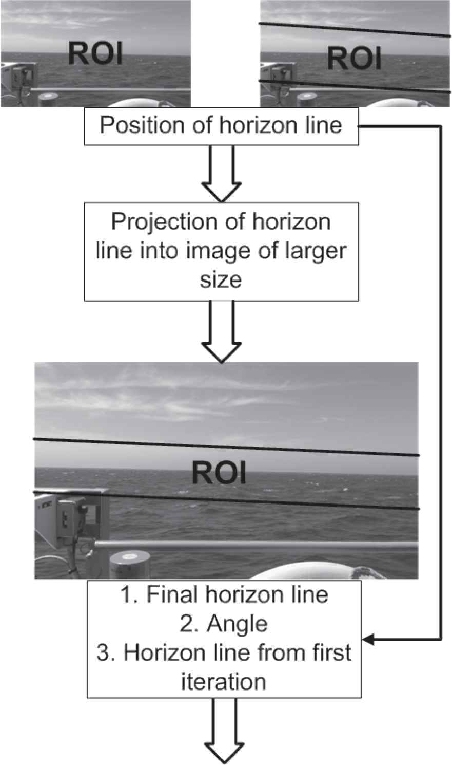
Operation of quick horizon line detection (QHLD) in two iterations (upper images are processed in the first iteration of the algorithm, left image corresponds to the very first run of the algorithm when even rough location of the horizon line is unknown whereas the right image is fed to the algorithm when a rough location of the line is already known, for example, in effect of previous run of the algorithm, the bottom full-size image is processed in the last iteration of the algorithm for accurate tuning of the horizon line location) [10].
To detect the HL inside the ROI, the QHLD compares brightness of potential HLs with the brightness of parallel lines lying one pixel above1, and the line characterized by the highest absolute difference in brightness is considered to be the HL. In the first iteration, the difference is calculated with a high accuracy, that is, for all pixels belonging to the compared lines, whereas in later iterations the difference is approximate and is calculated only for a portion of pixels [10].
3.2. Gradual Edge Level Decrease
The GELD is formally defined in Figures 2 and 3. It detects the HL based on the edge information, and the Sobel filter is used for that purpose. The HL is generated for a different strength of edge pixels—T, a different size of accepted holes between edge pixels—D, and a different method for searching HL pixels in the image—NP. To obtain images with a different strength of edges, first, they are subject to the Sobel filter and then they are thresholded with the parameter T—see Figure 4. This operation is performed by the function getSobel—see Figure 2. After generation of edges, the GELD tries to find a path between the leftmost and the rightmost columns of the image which leads through bright pixels. To this end, getHL function (see Figure 3) is used which implements two different strategies for generating a path, the function with the last parameter equal to 0 implements the primary strategy, whereas the parameter equal to 1 means the secondary one. First, the primary strategy is applied and if it fails, that is, the HL is not found, its secondary counterpart is run. If the algorithm cannot find any line for all Ts and Ds, it is assumed that the input image does not include the land, the HL is between the sea and sky.
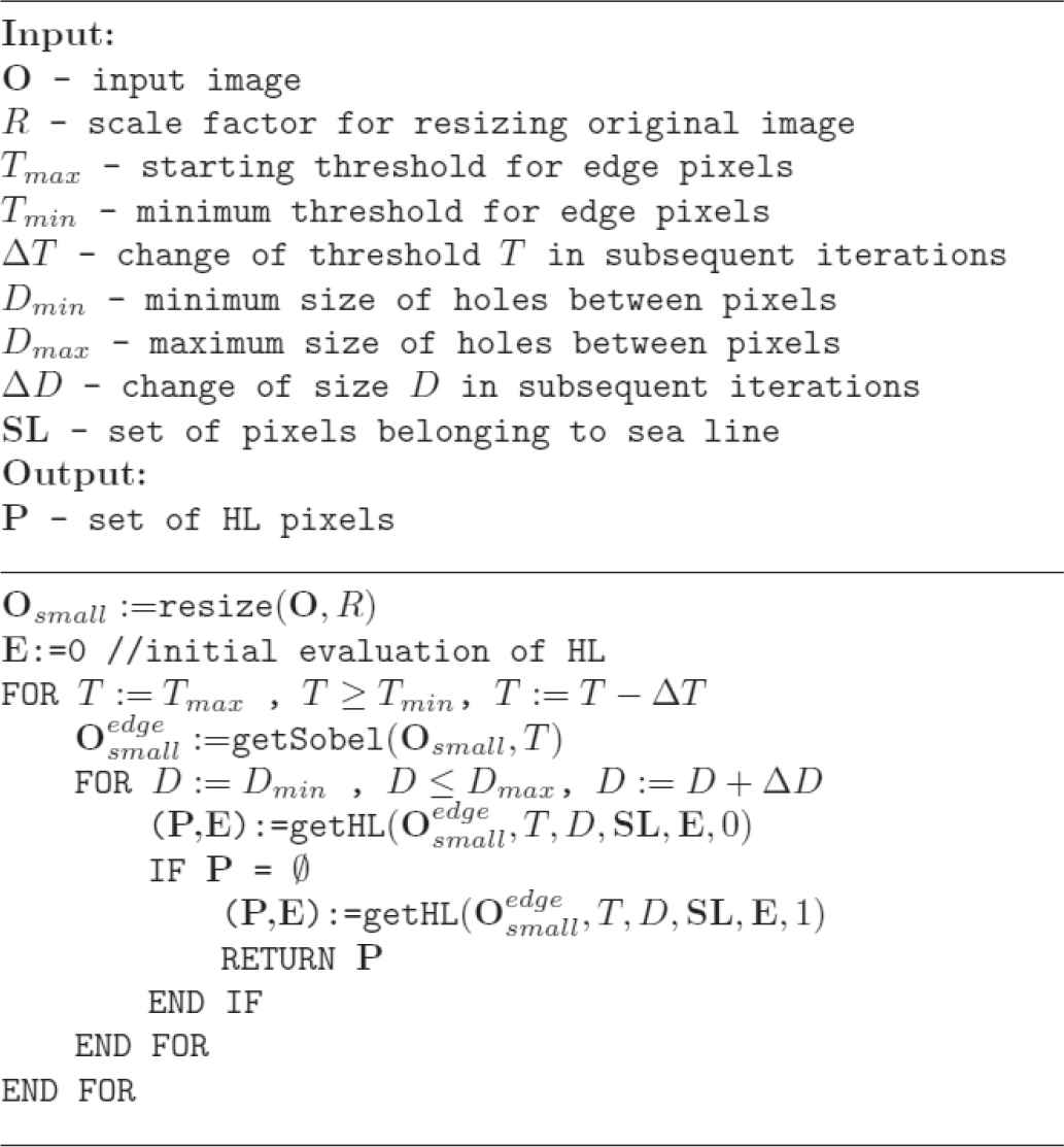
Pseudocode of gradual edge level decrease (GELD) working in one direction.
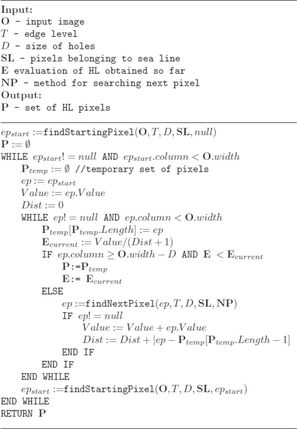
Pseudocode of getHL function.
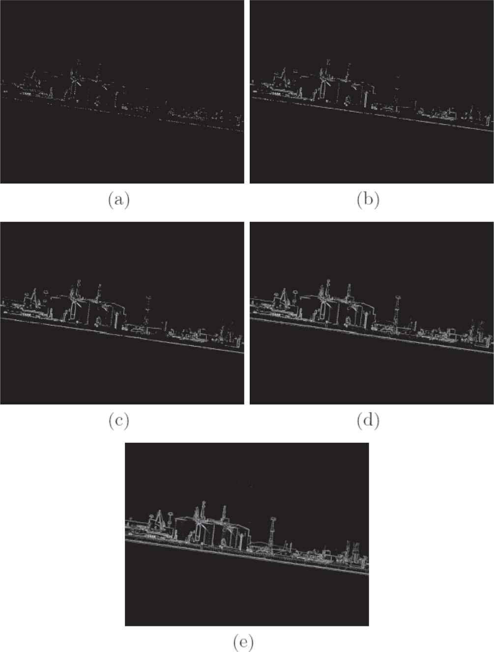
Images with different strength of edges that are applied in gradual edge level decrease (GELD).
In order to select the best HL out of all lines generated for different T and D, all lines are evaluated according to the following simple formula E = Value/ (Dist + 1), where Value is the total brightens of all pixels belonging the line, whereas Dist is the total distance between neighboring path pixels. During operation, the GELD maintains only one the best line, once a better line is found it replaces the previous one.
At first, the algorithm generates lines from the left to the right side of the image, if not found, it is repeated in the opposite direction. Such procedure sensitizes the algorithm to the land that occupies only a part of the image, either left or right. Unfortunately, the algorithm in the present form cannot detect the land situated only in the center of the image.
Each run of the getHL function begins with selecting a starting HL pixel located in the leftmost/rightmost column of the image. The function tries different starting pixels, all of them are situated above the SL, detected by the QHLD, and they are separated from each other by distance D. At first, the nearest pixel to the SL becomes a starting HL pixel, and in the case of failure (the HL is not found), a next edge pixel is selected. It is sought among pixels which are above the previous one and which are at least at a distance D from it. Searching for starting pixels according to the procedure described above is implemented in function findStartingPixel (see Figure 3).
Once the starting pixel is found its successor is sought at a distance at most D pixels. To this end, two different strategies can be used. The first one, which is the primary strategy, seeks the successor pixel along a predefined path. Initially, the neighboring column to the right/left is analyzed, from the top to the bottom, if it does not include any bright pixel, the algorithm moves to the next column, and so on (see Figure 5). The second strategy that supports the primary one in case of failure, returns the strongest pixel in the distance D from the current pixel, in this case, the whole pixel neighborhood has to be explored to find the successor. Searching for next HL pixel is implemented in function findNextPixel (see Figure 3).
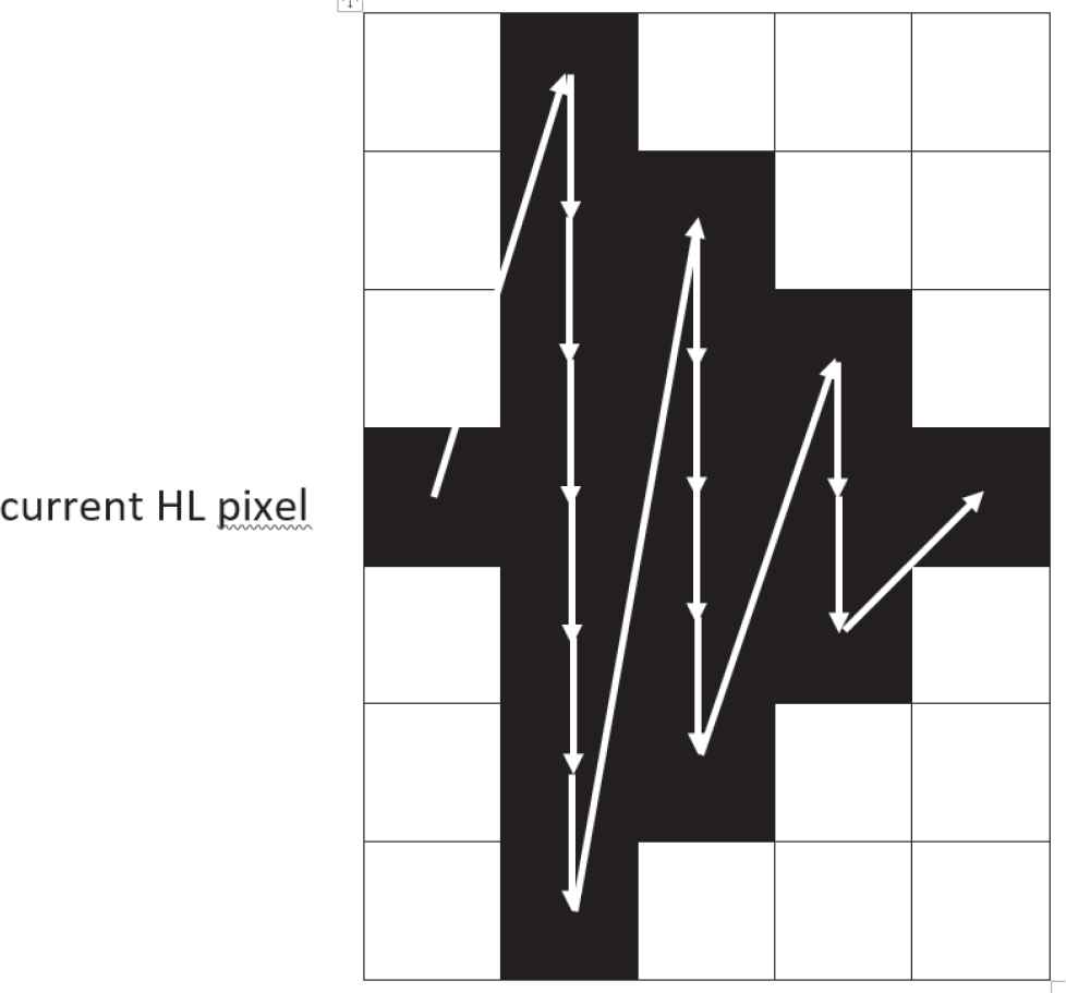
Path of searching for a successor edge pixel that is implemented in findNextPixel, the first edge pixel found along the path is returned.
In order to speed up the GELD, all its calculations are performed on smaller resized counterpart of the original image. A high speed of the algorithm is necessary because it is assumed that for estimation of the distance to the land for a given vehicle line of sight a number of images is processed and a final distance is an average of all individual measurements. What is more, in order to determine vehicle position, a number of distances is necessary, each one for a different line of sight. In consequence, the GELD together with the QHLD should be as quick as possible, they are allowed to make rare mistakes which in case of gross errors are easy to detect, their high speed and potential to make many measurements in a short period should, however, compensate occurrence of infrequent mistakes.
4. EXPERIMENTS
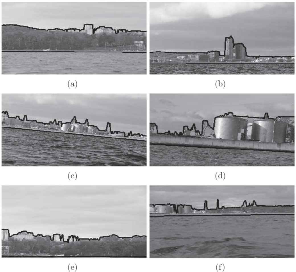
In order to verify effectiveness of the LDA, experiments were carried out with the use of 150 real images of Gdynia harbor and its neighborhood. They were recorded in different weather conditions and distances to the land: 60 images—a large distance to the land, 60 images—an average distance to the land, 30 images—small distance to the land, assignment of images to each group was subjective, example images are depicted in Figure 6. To test if the algorithm is also able to cope with images without visible land, the set of testing images were supplemented with ten extra images recorded at open sea, their examples are presented in Figure 7.
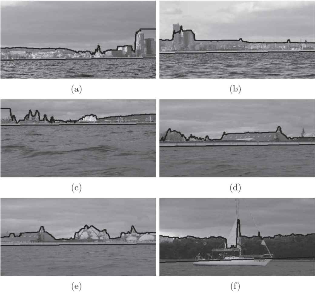
To verify effectiveness of the algorithm, location of SL and HL lines was visually evaluated by a man-expert. Given that the target application of the LDA is estimation of the distance to the land based on size of the land area in a sequence of images, with the effect that accuracy of the algorithm does not have to be at a pixel level, instead of automatic verification of the algorithm, subjective human-made evaluation was performed. The following grades could be assigned to SL and HL lines: SL = {A—a perfect line, D—a wrong line}, HL = {A—a perfect line, B—an almost perfect line with single deviations from the perfect line, a line with sufficient accuracy, the estimated size of the land determined by means of the line does not significantly differ from the correct size, D—wrong line}. Example images with different HL grades are presented in Figure 8.
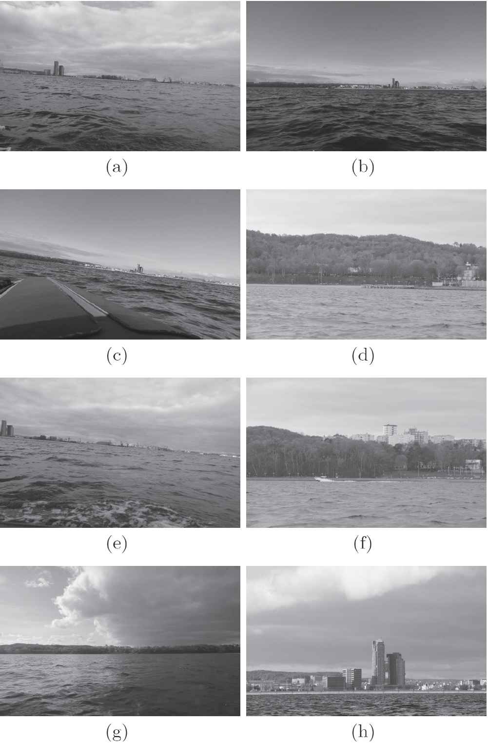
Example images with visible land that were used in experiments.
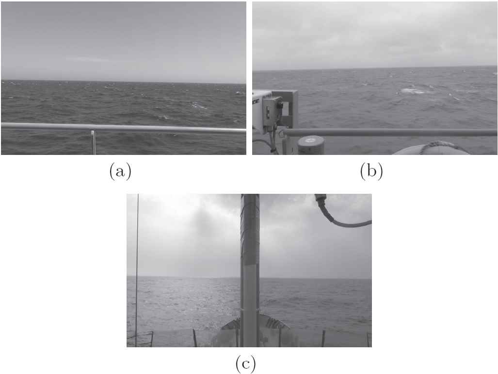
Example images without visible land that were used in experiments.
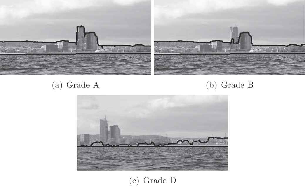
Example images with different evaluation.
In the experiments, a simplified variant of the QHLD was applied. The original variant is run in two or three iterations with the purpose to accurately determine location of the HL in the image, and then, spatial orientation of the camera, and in consequence a ship. Accurate measurements are, in this case, necessary for right operation of different ship systems that require accurate information about ship spatial orientation. Meanwhile, in the problem of land detection, accurate determination of SL and HL is not so important as speed of the algorithm and that is why the decision was made to apply in the experiments a quicker single-iteration variant of the QHLD.
Verification of LDA performance was preceded by tuning the algorithm parameters with the use of 30 test images. In effect, the following parameter setting was considered to be the most effective: R = 0.3, Tmax = 100, Tmin = 20, ΔT = 20, Dmax = 30, Dmin = 10, ΔD = 10. Settings for R for both the QHLD and GELD were the same. R was the only tunable parameter of the QHLD, the remaining algorithm parameters were the same as those applied in the experiments reported in [10].
Segmentation approach based on k-means and Gaussian mixture model (GMM) [21, 22] combined with the QHLD was used as a point of reference for the LDA. Since the images used in the experiments were unlabeled, detection of the land was impossible by means of deep learning and classification techniques. They both use supervised learning to prepare “land detectors,” mainly in the form of neural networks, which means that they need labeled data in the training process. Since, as mentioned above, such data were unavailable, the above techniques could not be tested and compared to the LDA.
In order to differ the land from other content of the image, k-means and GMM segmentation had to be supported by extra processing of segmented images. Because the sea segment is very hard to isolate from other elements of the image, this task was assigned to the QHLD. This way, only parts of images above the SL were subject to segmentation. In the experiments, an approach with many segments (clusters) was applied (like in [9]) with the purpose to extract thin land segments. Moreover, to make them flat and horizontal, segmentation was performed in 4D space, that is, in 3D RGB color space extended by the vertical coordinate of the pixels.
After the segmentation, a number of segments were determined without indication which of them corresponds to the land. In order to select the land segment from the set of all extracted segments, fourth coordinate (number of image row) of segment centroids was tested, and a segment whose centroid lied directly above the SL was considered to be the land segment. Since the selected segment very often included single “foreign” pixels from other segments, all pixels inside the area determined by border land pixels were classified as the land. All the above process of extracting the land from the image by means of k-means/GMM–QHLD method is explained in Figure 9.
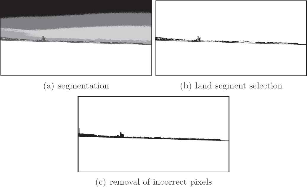
Operation of k-means-quick horizon line detection (QHLD).
Results of all the experiments are summarized in Tables 1 and 2. They do not include results of the QHLD because the SL line was incorrect only in one case presented in Figure 10. In the remaining 149 cases, the SL line was determined properly. Even though the QHLD was designed for working at open sea, it showed effectiveness also in other more challenging conditions. As it turned out, an additional content of images, apart from the sea and sky, does not have a negative influence on algorithm performance. What is more, a simplified variant of the algorithm with only one iteration appeared to be sufficient to successfully perform the task.
| Grade/Distance to Land | LD(%) | AD(%) | SD(%) | T(%) |
|---|---|---|---|---|
| A | 83 | 42 | 10 | 52 |
| B | 17 | 58 | 58 | 40 |
| D | – | – | 32 | 8 |
GELD, gradual edge level decrease; LD, large distance; AD, average distance; SD, small distance; T, total.
Results of GELD.
| Grade/Distance to Land | LD(%) | AD(%) | SD(%) | T(%) |
|---|---|---|---|---|
| A | 40 | 27 | 6 | 28 |
| B | 47 | 53 | 57 | 51 |
| D | 13 | 20 | 37 | 21 |
QHLD, quick horizon line detection; LD, large distance; AD, average distance; SD, small distance; T, total.
Results of k-means-QHLD.
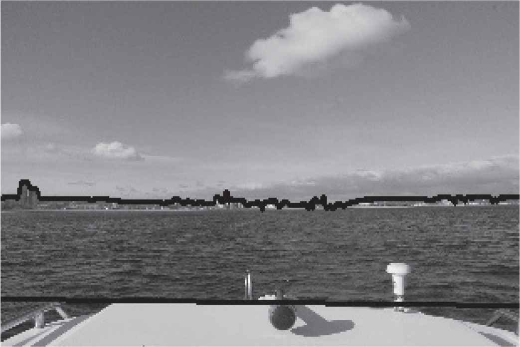
Image with incorrect sea line (SL).
The tables also do not include results of GMM segmentation. As it appeared, k-means segmented images in a more effective way from the points of view of land extraction than GMM, and that is why the results of the latter segmentation method were neglected in the paper.
The above tables show that the method proposed in the paper is generally more effective in extracting the land from marine images than the one relying on k-means segmentation. In the former case, as many as 92% of HLs, that is, the ones with grade A–C, would enable estimation of the distance to the land without gross errors. Only 8% of HLs should be rejected. In the latter case, 79% of land segments seem roughly correct, the remaining ones would result in serious errors in the distance estimations. Example results of application of both rival methods are depicted in Figures 11–14.
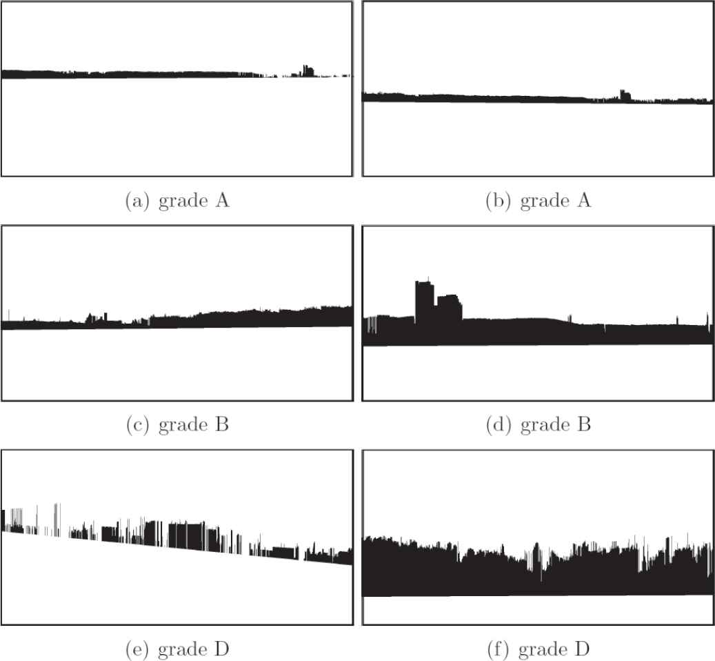
Images with grade A produced by land detection algorithm (LDA).
Images with grade B produced by land detection algorithm (LDA).
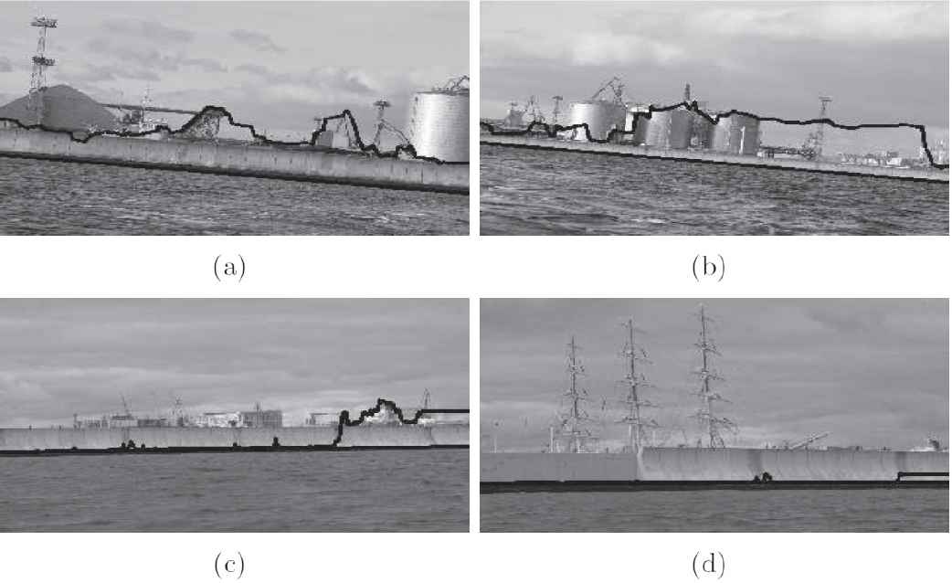
Images with grade D produced by land detection algorithm (LDA).
Land extracted by k-means-QHLD.
In both cases, reducing the distance to the land makes correct work of both methods difficult. Presence of more details in images, elements of harbor infrastructure, piers, buildings, threes, and so on, entails possibility to lead the HLs in many different ways, very often in an improper one. A small distance to the land also increases size of the land area in the image. In consequence, it is represented by many different k-means segments which hinders its correct identification.
However, increase of the distance considerably improves the results. For a large distance, 100% of HLs and 87% of k-means land segments are proper. Even “roughness” of the HL caused by cranes, trees, and other high protruding elements of the scene are not an obstacle in generating correct HLs and land segments.
Analysis of HL parameters revealed that, in most cases, the perfect lines with the grade A are generated for D = 10 and T = 40, 60, 80. For higher values of D (20 or 30), quality of the lines deteriorates, they lose smoothness, include sudden bounds, sometimes, they completely do not reflect true HLs. However, as it appeared, the lines with D = 20, 30 were, in most cases, optimal only if the GELD did not find any line for D = 10. There are only a few HLs with grade A and D = 20, 30 which got higher evaluation E than their equivalents with D = 10.
The experiments with images that do not contain the land showed that HLs are generated only for T = 20 (see Figure 15), higher values of that parameter that require stronger edges cause the lines not to appear. In the case of images with the land visible, the proper HLs are, in majority of cases, produced for T ≥ 40, which means that in order to prevent the GELD against improper operation at open sea, it is only enough to increase Tmin to value 40.
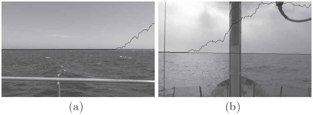
Example sea line (SL)/horizon line (HL) generated for images without land visible.
5. SUMMARY
In the paper, the algorithm for detection of land areas in marine images is proposed. To perform the task, the algorithm extracts two lines from images, that is, the SL and HL. They both are borderlines between semantically different regions, the latter one divides images into the sea and the land region, whereas the former one into the land and the sky region. The area between both lines is considered to be the land.
In order to extract the abovementioned lines, the algorithm, called LDA, exploits two other algorithms, that is, QHLD and GELD. The task of the first one is to detect the SL, whereas the second one is applied for the HL extraction. The QHLD was originally designed for detecting HLs in marine images without land content and it is detailed in [10]. In turn, the GELD belongs to the class of edge-based algorithms and to the best knowledge of the authors it can be recognized as a variation of the method proposed in [13].
Apart from the presentation of the LDA, the paper also reports verification experiments on real marine images. As it appeared, the proposed algorithm is an effective tool for the land detection. In the experiments, the land was properly detected in majority of testing images, what is more, the algorithm also showed that it is able to identify situations when the land is not visible in the image.
In spite of the fact that the algorithm was originally designed for autonomous marine vehicles and navigation purposes in GPS denied environments its effectiveness can be also used for labeling images. As mentioned above, the algorithm properly detected the land in majority of cases, its effectiveness was not ideal. However, the fact that there were few images in which the land was generated incorrectly does not mean that the algorithm cannot find proper lines in these images. To find them it is simply enough to manually tune its parameters D and T. Since the algorithm is very quick, its tuning to each single image can be almost immediate which means that labeling procedure on a number of images can be also performed very quickly.
ACKNOWLEDGMENTS
The paper is supported by European Defense Agency project no. B-1452-GP entitled “Swarm of Biomimetic Underwater Vehicle for Underwater ISR” and Research Grant of Polish Ministry of Defense entitled “Optical Coastal Marine Navigational System.”
Footnotes
gGray-scale images are used.
REFERENCES
Cite this article
TY  - JOUR
AU  - Tomasz Praczyk
PY  - 2018
DA  - 2018/12/17
TI  - Detection of Land in Marine Images
JO  - International Journal of Computational Intelligence Systems
SP  - 273
EP  - 281
VL  - 12
IS  - 1
SN  - 1875-6883
UR  - https://doi.org/10.2991/ijcis.2018.125905640
DO  - 10.2991/ijcis.2018.125905640
ID  - Praczyk2018
ER  -