
An Empirical Study for Enhanced Software Defect Prediction Using a Learning-Based Framework
Corresponding author. Email: trli@swjtu.edu.cn
- DOI
- 10.2991/ijcis.2018.125905638How to use a DOI?
- Keywords
- Software defect prediction; Feature selection; Data sampling; Noise filtering
- Abstract
The object of software defect prediction (SDP) is to identify defect-prone modules. This is achieved through constructing prediction models using datasets obtained by mining software historical depositories. However, data mined from these depositories are often associated with high dimensionality, class imbalance, and mislabels which deteriorate classification performance and increase model complexity. In order to mitigate the consequences, this paper proposes an integrated preprocessing framework in which feature selection (FS), data balance (DB), and noise filtering (NF) techniques are fused to deal with the factors that deteriorate learning performance. We apply the proposed framework on three software metrics, namely static code metric (SCM), object oriented metric (OOM), and combined metric (CombM) and build models based on four scenarios (S): (S1) original data; (S2) FS subsets; (S3) FS subsets after DB using random under sampling (RUS) and synthetic minority oversampling technique (SMOTE); (S4) FS subsets after DB (RUS and SMOTE); and NF using iterative partitioning filter (IPF) and iterative noise filtering based on the fusing of classifiers (INFFC). Empirical results show that 1. the integrated preprocessing of FS, DB, and NF improves the performance of all the models built for SDP, 2. for all FS methods, all the models improve performance progressively from S2 through to S4 in all the software metrics, 3. model performance based on S4 is statistically significantly better than the performance based on S3 for all the software metrics, and 4. in order to achieve optimal model performance for SDP, appropriate implementation of the proposed framework is required. The results also validate the effectiveness of our proposal and provide guidelines for achieving quality training data that enhances model performance for SDP.
- Copyright
- © 2019 The Authors. Published by Atlantis Press SARL.
- Open Access
- This is an open access article distributed under the CC BY-NC 4.0 license (http://creativecommons.org/licenses/by-nc/4.0/).
1. INTRODUCTION
A software defect refers to an incorrect step, process, or data definition in a computer program [1]. A defect in software causes it to output wrong results and respond in ways not expected. Consequently, the target of software defect prediction (SDP) is to enhance software quality through prompt identification of fault-prone (FP) modules using metric-based classification [2]. To minimize maintenance cost for a quality product delivery, SDP attempts to predict the number of defects as well as the fault-proneness of system components before they are utilized. As asserted by Fagan [3], early detection is important due to the comparative advantage of minimized correction cost. To develop SDP models, prior experience of system components is required to identify and predict FP modules.
In this regard, historical software metrics and fault data serve as primary input to the models. These models are used subsequently to identify FP or non-FP (NFP) modules to estimate the quality of a software component. The practical approach to prediction of FP software modules is necessary for appropriate testing to reduce costs and aid in the efficient management of resources by software developers. This can also result in significant improvement in software quality and culminate in user confidence and reliability in the supply chain. To identify FP software module, binary prediction models are mostly used on the metric type in question to identify a module as either defective or otherwise [4].
In machine learning domain, a learner is induced on the set of training data which functions based on a set of rules to discriminate between fault and nonfault. Therefore, the ability of these learners to classify a module is primarily a function of the quality of training dataset. However, data collection comes with several challenges in generation, processing, storing, and retrieval. These processes according to [5–8] have a higher potential of causing data quality difficulties such as feature redundancy and irrelevance, data example conflict, class imbalance, the presence of noise, and abnormality.
The common challenges in SDP are high dimensionality, class imbalance, and class mislabels. High dimensionality refers to the situation where training data has an unduly higher number of attributes with which an induced learner is trained for classification. Over the years, several successful studies have been conducted on the impact of high dimensionality in training data on learning performance. By using feature selection (FS) to eliminate redundant and irrelevant attributes, classification models would take a limited time to learn, and these models would perform better in predicting defective modules relative to those constructed using entire features [8]. Again, in a study conducted by Chubato et al. [9] in which a combine learning-based framework was proposed to improve SDP, it was pointed out that the software testing prefers to use fewer software metrics.
Also, when the dataset is skewed toward a specific class of instances, class imbalance results. Class imbalance is common among different applications including software quality evaluation. However, an imbalance in data was identified to pose a significant challenge to learners by Khoshgoftaar et al. [10] in which a process for best FS was proposed to improve model performance when dealing with imbalance data. This was the case, especially in software defect datasets which are often used for training in classification for SDP. The imbalanced data problem occurs when the examples in one class significantly outnumber the examples of the other class. The minority class is usually the one that represents the concept to be learned. Relating to our field of study, FP modules which represent the target concept are always relatively lesser than NFP. The difficulty of learning from imbalance dataset stems from the concept of learning where most of the standard learning algorithms consider the training set balance.
When this condition is not satisfied, they tend to be biased toward the majority class and consequently generate a suboptimal model which provides sufficient coverage for the majority class, whereas the minority class is often misclassified. These kinds of predictions are considered inefficient especially for software practitioners because their target concept is FP modules which constitute the minority. Considering the impact, many studies have been successfully conducted over the years, and several solutions such as data balance (DB), algorithmic modification, and cost-sensitive learning proposed to deal with the challenges imposed on standard learning algorithms [11].
Class noise in the dataset is another major problem in SDP as it is known to influence the way any data mining system performs [12]. Class noise refers to class mislabel. In this regard, real-world data is not immune to noise for the reason that data collection and preparation processes expose them to class mislabel and the consequences are grave in building a defect prediction model. For this reason, more effort is required to mitigate the effects. Several studies had consistently confirmed that a classifier performance would be adversely impacted when the training dataset used to construct it is corrupted.
Class noise (or labeling errors) is produced when the examples are labeled with the wrong classes. In SDP, class noise is a critical issue toward fault prediction as it affects the accuracy of classification of software modules. Training dataset incorporates a considerable amount of inconsistencies in expected syntax, semantics, or values, which result in poor quality data. This can affect both FP and NFP modules, dependent variables. This assertion is confirmed in a study by Khoshgoftaar et al. [13], and they further stated that inducing learner on noisy training data could produce inaccurate predictions because the decision is based on incorrect information. Noise filters (NFs) are designed to eliminate noisy examples in training set to improve classification performance.
This paper as an extension of our previous research work [14] examines the learning impact of applying different preprocessing methods on a variety of classification algorithms including Nave Bayes (NB), random forest (RaF), K-nearest neighbors (KNN), nultilayer perceptron (MLP), support vector machine (SVM), decision tree (J48), decision stump (DSt), and the logistic regression (LR). The objective of this work is to analyze the learning influence of the data preprocessing that jointly apply FS, DB, and NF on classification performance for SDP as against other preprocessing methods in the literature. From a real-world software quality dataset, we derive 12 datasets categorized under static code metrics (SCM), object oriented metrics (OOM), and combined metrics (CombM) with different levels of data dimensions, imbalance, and noisy. We apply eight FS techniques to these datasets combined with two different forms of sampling, and NF to build the eight classifiers under different learning scenarios. We examine the interaction between the choice of FS, classifier, sampling, and NF technique on each of the software metrics. In this work, we address the following research questions:
What is the relative learning impact of the preprocessing method that jointly applies FS, DB, and NF versus those that apply FS, FS followed by DB, and no preprocessing? Which has a more positive impact on the performance of the different classification algorithms?
How does the average classification model built on different software metrics react to the application of different data preprocessing techniques? Do the data preprocessing method lead to better performance when the model built is based on one software metric than the other?
Do some sampling methods based on FS subset work better when used in combination with specific classification algorithms?
When the data is highly imbalanced or very noisy, do certain sampling and NF techniques perform better than others?
How do classification algorithms perform at different levels of class imbalance and noise after sampling and NF techniques have been applied to the data? When the data is high dimensional, highly imbalanced, and very noisy, do certain classification algorithms perform better than others?
The rest of the research is arranged as follows: Section 2 provides the related work. Section 3 describes the proposed framework, including more detailed information about the FS techniques, DB, NF, learners, performance index, and statistical test which are applied in this work. Sections 4 presents the experimental design. The resulting analysis and discussion are reported in Section 5. Finally, the conclusion and future work are given in Section 6.
2. RELATED WORK
For more insight into previous works relating to the topic, we present a literature review on past studies that addressed classification problems to build SDP models. The quality dataset is crucial for enhanced learning in SDP. Many studies apply different methods including FS to ensure the selection of most relevant feature subset for constructing prediction model with the view to enhance learning performance for classification and prediction for SDP. In a classical work on an empirical study of feature ranking techniques for software quality prediction by Khoshgoftaar et al. [15], seven filter based feature ranking techniques for comparison using 16 software datasets were examined. Their proposed ensemble learning architecture considered various basic classifiers including NB, artificial neural network (ANN), KNN, SVM, and LR models. The experimental results demonstrated that classification performance based on information gain (IG) and signal noise ratio (SNR) FS techniques improve significantly relative to the rest of the FS techniques.
In a similar study to improve learning performance, Xu et al. contended that the performance of models built for defect prediction is affected by high dimensionality in training data. To justify their claim, an extensive study was conducted [16] to investigate the impact of 32 FS methods on defect prediction over several datasets. The experimental results showed that the effectiveness of the selected FS methods varies significantly over different datasets. These results did not only confirm their claim but also demonstrate that the choice of software metric is essential to improve learning performance for SDP.
Furthermore, it has been observed that imbalance distribution of class examples is counterproductive for the learning performance in SDP. Several studies, including Wang and Yao [17], investigated different types of class imbalance learning methods and proposed a dynamic version of AdaBoost.NC which adjusts its parameters automatically during training for a more balanced class distribution in the training set. The experimental results demonstrated an enhanced performance by their approach.
Other schools of thought are of the view that mislabeled class examples in training data impede learning performance and proceed to design noise filters using ML techniques to reduce such impact for SDP. For instance, Khoshgoftaar and Rebours [13] proposed an iterative-partitioning filter (IPF) NF technique to improve software quality prediction. It removes the noisy data iteratively using several classifiers built with the same learning algorithm. Their proposal experimented with several datasets, and the results confirmed the predictive performance of models built on filtered training datasets is better than those built on the noisy training set. In the same line of thought, Sáez et al. [18] proposed the Iterative NF based on the Fusion of Classifiers (INFFC) which combines three different NF paradigms. These include the usage of ensembles for filtering, the iterative filtering and the computation of noise measures based on the fusion of the predictions of several classifiers. Their proposed method was applied to different datasets from KEEL-Dataset, and UCI repositories and the improved learning performance was reported.
Although these techniques, when applied independently, improve performance as cited in the literature above, it is important to state that their synergistic effect may vary significantly as far as SDP. Other research, under this idea, adopts a combined learning approach in which various techniques are sequentially executed during preprocessing to enhance data quality further. Along this line, Khoshgoftaar et al. [19] applied FS and DB to examine four possible situations (S): 1. FS based on primary data, and using balanced data for modeling, 2. FS based on primary data, and using primary data for modeling. 3. FS based on balanced data, and modeling based on balanced data, and (4) FS based on balanced data, and modeling based on primary data. Their experimental results confirmed that FS using balanced data gives better performance than FS based on primary data.
In a similar study, Shanab et al. [20] discovered that models under S3 have higher performance than S2. Furthermore, Khoshgoftaar et al. [21] also identified class imbalance and high dimensionality as in the previous study mentioned above. They instead proposed an iterative FS approach, which repeatedly applies data sampling followed by FS and finally performs an aggregation step to combine the ranked feature lists from the separate iterations of sampling. This approach was devised to attain a list of ranked features which is particularly efficient on the more balanced dataset emerging from sampling while decreasing the risk of losing data during the sampling step and missing essential features. The study was carried out using three groups of datasets with different levels of class balance. The results demonstrated improved learning performance
Again, Liu et al. [22] combined FS with DB using sampling methods with the goal to decrease the total number of examples rather than handling class imbalance. Handling the same problem of imbalance and high dimensionality for enhanced software quality, Khoshgoftaar et al. [8] applied data sampling collectively with FS. The empirical results demonstrated that it is more efficient using FS with data sampling relative to using each technique separately. This assertion was confirmed by Chubato et al. [9], in which they developed a combined learning framework which includes FS together with DB to improve learning performance for SDP. Based on the experimental results, they stated that their framework could guarantee improved learning performance for SDP.
To the best of our experience, over the years, those difficulties (class imbalance, high dimensionality, and noisy data) have got extreme concentration. The huge amount of study has been done to understanding, treating, and mitigating each problem independently and in the rare case, a combination of FS and DS techniques. Limited work is done on the datasets that are characterized by having these difficulties together. Thus, the purpose of this study is to develop a framework which improves training dataset quality to enhance the performance of SDP.
3. EXPERIMENTAL METHODOLOGY
This section describes the proposed framework (taken into account the datasets, FS, DB, NF, learning algorithms, and evaluation criteria) and experimental design.
3.1. Hypothesis
If a data preprocessing approach combines FS, DB, and NF, the classification performance of the resulting model for SDP in the three software metrics, will be better than one that does not.
3.2. The Proposed Framework for SDP
In this section, we describe the proposed framework for SDP in brief as shown in Fig. 1. The software metrics considered for this study are independently treated following the procedures outlined. To test the study hypothesis, we build and assess model performance following four scenarios: 1. using normal datasets for training, 2. learning from FS subsets, 3. learning from balanced FS subset of data, and 4. learning from noise filtered, balanced FS subset. For the analysis of learning performance under the given scenarios, we consider average AUC measure for each scenario.
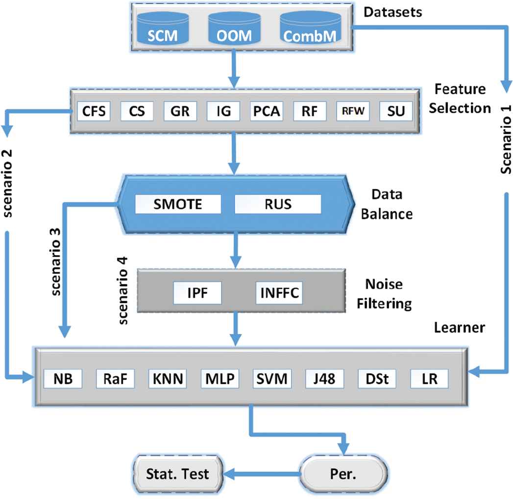
A framework to enhance software defect prediction (SDP).
3.2.1. Software metrics
SCM: The SCM results from attempts by McCabe and Halstead to objectively characterize code features that are associated with software quality. Their measures are based on the module, where a module refers to the smallest unit of functionality. McCabe [23] claimed that codes with complex pathways are more prone to error. Therefore, his metrics reveals the pathways within a code module and composes of four software metrics, for example, cyclomatic complexity (CC), essential complexity (EC), design complexity (DC), and lines of code (LOC). Whereas, Halstead argued that code that is complex to read is more likely to be fault-prone [24]. Halstead metrics assess the complexity by counting the number of concepts in a module. For instance, the number of unique operators/operands. The Halstead metrics fall into three groups, that is, the base measures (BM), the derived measures (DM), and LOC measures (LOCM). The worth of using SCM to build models for SDP has been empirically illustrated by Menzies et al. [24], who claimed that SCM are useful, easy to use, and extensively used.
Object-oriented metrics (OOM): According to Chidamber et al. [25], object-oriented (OO) software metrics applied at a class-level can be classified under three phases of OO design processes. The first phase is identification of classes (IoC) which comprises weighted methods for class (WMC), depth of inheritance tree (DIT), and number of children (NOC); the second phase is semantics of classes (SoC) which comprise WMC, response for class (RFC), and lack of cohesion of methods (LCOMs); and the final stage is relationships between classes (RBCs) which includes RFC and coupling between objects (CBO).
CombM: D’Ambros et al. [26] developed the combined form metrics (AEEEM). It combines six different groups of software metrics containing 61 metrics: process metrics, previous defects metrics, source code metrics, the entropy of changes, churn (source code metrics), and entropy (source code metrics)
3.2.2. Feature selection
Selecting useful features has been found to be beneficial for the improved quality of training dataset in SDP. In most cases, the classification accuracy using the reduced feature set equaled to or was better than using the complete feature set [27]. Therefore, this study employs eight widely used FS techniques (FST). Each of these FST has been proven useful in [24, 28]. The use of different FST would help us to attain the objective of identifying which FS approach in combination with DS and NF techniques is/are most suitable for the given software metric.
Correlation feature selection (CFS): CFS can be used to rank features according to a correlation based on the heuristic evaluation function [29]. The evaluation function is a bias toward subsets that contain features that are highly correlated with the class and uncorrelated with each other. Irrelevant features are ignored because they are evaluated to have low correlation with the class. Features highly correlated with one or more of the remaining features are regarded as redundant and screened out. The selection of features, therefore, is purely based on the extent to which they predict classes in areas of the instance space not already predicted by other features. The evaluation function is represented by
Here,
The
Chi-square (CS): Given a feature f, CS is a nonparametric statistical measure that examines the correlation between the distribution of f and that of class [30]. It can be computed by the following formula:
Here r is the number of distinct values of the feature, nc denotes the number of classes (for a binary classification as in this study, nc is 2), Oi,j is the observed number of instances with the feature value i in the class j, and Ei,j is the expected (i.e., mean) number of instances with any value i in the class j.
IG: Given a feature f, IG measures the amount of information f can provide to the class [31]. This information can be used to select the optimal feature sets. IG measure can be computed by the following formula:
H(X|Y) computes the conditional entropy which quantifies the uncertainty of X given the observed variable Y (i.e., the feature). Let p(x|y) denote the posterior probability of x given the value y of Y. H(X|Y) can be computed by the following formula:
Gain ratio (GR): GR compensates a drawback of IG and penalizes multivalued features to handle the drawback [24]. The GR is defined accordingly as
Principal components analysis (PCA): The PCA approach [30] can be used to reduce the dimensionality of the input features. In general, the PCA technique transforms n vectors (x1, x2, … xi, …, xn) from a d-dimensional space to n vectors (x′1, x′2, … x′i, …, x′n) in a new, d’-dimensional space.
ReliefF (RF, RFW): RF proposed by Kira and Rendell in 1992 [32] is an instance-based feature ranking technique. Its strengths are that it is not dependent on heuristics, runs in low-order polynomial time, and is noise-tolerant and robust to feature interactions, as well as being applicable for binary or continuous data. Kononenko et al. proposed a number of updates to RF while pointing out that it can measure how well a feature differentiates instances from different classes by searching for the nearest neighbors of the instances from both the same and different classes [33]. The RF evaluation function is represented below.
Symmetric uncertainty (SU): SU can be used to calculate the fitness of features for FS by calculating between feature and the target class according to [34]. Importance of features is based on the value of SU computed. The higher the value, the more importance is attached to the feature. SU is defined as follows:
In which H(X) is the entropy of a discrete random variable X. If the prior probability of each element of X is p(x), then H(X) as defined in Equation (4).
3.3. Data Balance
The primary challenge of learning from imbalanced datasets is the tendency of the standard classifier to disregard the importance of the minority class by virtue of its rarity resulting in classification bias toward the majority class. The approach to solving the challenges imposed by class imbalance, according to a study by Catal et al. [35] is mainly categorized into data sampling, cost sensitive learning, and ensemble learning methods. In this research, we adopt the SMOTE and RUS methods together with other machine learning approaches to improve learning performance for classification in SDP, consistent with previous research [36].
RUS mitigates the difficulty of class imbalance in a dataset by randomly dropping examples of the majority class which enhances learning performance. It removes data from the original dataset such that |D| = |Dmin| + |Dmaj| − |E|, where removed samples come from a randomly selected set of majority class examples in Dmaj resulting in D. Consequently, undersampling readily gives us a simple method for adjusting the balance of the original dataset D.
In a similar narration in [37], they stated that SMOTE is a successful method in several areas and applications. It can also be said to be the base foundation for all oversampling methods [38]. Instead of duplicating the minority class samples, SMOTE works on creating new synthetic examples in minority classes. The synthetic examples are generated in feature space rather than data space. The SMOTE samples are linear combinations of two similar samples from the minority class (X and X′) and are defined as S = S + u.(X′ − X) with 0 ≤ u ≤ 1. X′ is randomly chosen from the K minority class nearest neighbors of X. The newly built examples decrease rarity in the minority and make it fuller and more general. This study adopts (35:65) minority:majority ratio as imbalance threshold as proposed in [39].
3.4. Noise Filtering
To eliminate noisy examples in the training set, NF are designed. Different studies applied different filtering algorithms and reported insightful findings. This study choses to apply IPF and INFFC method on the basis of their wide usage in the literature and the technique adopted in noise elimination.
IPF resulting from the brilliant work of [13] partitions the training dataset into n subset, and the model is built on each subset and multiple iterations performed. Then, an instance is identified as noisy if it is mislabeled by a definite number of iteration.
INFFC developed in a study conducted by Sáez et al. [18] also follows a similar procedure as in IPF except that INFFC considering filtering techniques based on the usage of multiple classifiers. Three steps are carried out in each iteration. First, preliminary filtering is performed with an FC-based filter which considers the three classifiers (C4.5, 3-NN, and LR)). This first step removes a part of the existing noise in the current iteration to reduce its influence in posterior steps. More specifically, noise examples identified with high confidence are expected to be removed in this step.
Then, another FC-based filter is built from the examples that are not identified as noisy in the preliminary filtering to detect the noisy examples in the full set of instances in the current iteration. New filtering, which is built from the partially clean data from the previous step, is applied over all the training examples in the current iteration resulting into two sets of examples: a clean and a noisy set. This filtering is expected to be more accurate than the previous one since the NFs are built from cleaner data. Finally, to control the noise sensitivity of the filter, a noise score is computed over each potentially noisy example from the noisy set obtained in the previous step to determine which ones are finally eliminated. Noisy examples are only removed if they exceed a noise score metric.
3.5. Learners
We adopt the eight widely used supervised learning techniques in this study. These include NB, RaF, KNN, MLP, SVM, J48, DSt, and LR. The WEKA tool is used to instantiate the different classifiers. Parameter settings that ensure optimal performance are specific to different learning algorithms. Thus, this study applies the following configurations to the learners based on preliminary investigation:
Regarding the NB learner, we set the use Kernel Estimator to true in order that a kernel estimator for numeric attributes is used rather than a normal distribution. For the RaF learning algorithm, we alter the default value assigned to numTrees from 100 to 200. This modification increases the number of trees to be generated to get the better and more reliable estimates from out-of-bag predictions. Regarding higher values assignment to numTree, the concerns expressed in other studies about computation time has been considered in selecting this value. In the case of the KNN learning algorithm, the distanceWeighting parameter is set to Weight by 1/distance, the kNN parameter is adjusted to 5, and the crossValidate parameter is tuned to true. Considering the MLP, we set the hiddenLayers parameter to 3. This means that we define a network with one hidden layer containing three nodes. The validationSetSize parameter is also adjusted to 10. In this way, the MLP classifier leaves 10% of the training data aside for use as a validation set to determine when to stop the iterative training process. Two configurations are made for the SVM: the complexity constant c is set to 5.0, and build Logistic Models is set to true. In his study, we turn on (set to true) the useLaplace parameter for J48 to improve the probability estimates. And finally, with LR, we set errorOnProbabilities to True and useCrossValidation to false, to minimize the root mean squared error.
3.6. Performance Index
The area under the receiver operating characteristics curve (AUC) is the most suitable metric used to properly evaluate performance when imbalanced data is presented with unequal error cost [40]. The receiver operating characteristic (ROC) curve plots true positive rate on the y-axis against the false positive rate on the x-axis. The curve indicates the trade-off between detection rate and false alarm rate. Thus, this curve shows the performance of a classifier across the entire range of possible decision thresholds and accordingly does not assume particular misclassification costs or class prior probabilities. The AUC, which is calibrated over the range of 0 to 1, provides a single numerical metric for evaluating model performances. Higher values refer to better model performance and vise versa.
4. EXPERIMENTAL DESIGN
In this work, we partition data by implementing 10-fold cross-validation. Each dataset is randomly divided into ten respectively exclusive subsets (the folds) of about the same size. For ten times, nine folds are selected to train the models, and the remaining fold is used to test them. The performance of all learners is assessed toward any software defect dataset. To create and examine empirical results, we use WEKA version 3.6.13, MATLAB R2016a, KEEL software tool, and IBM SPSS Statistic23. AUC is adopted as an evaluation metric for leaning performance. Considering the objectives set for this study, we follow four scenarios to train and create the classification models.
Initially, we treat multiple software metrics individually and build classification models using eight most frequently used ML algorithms (NB, RaF, KNN, MLP, SVM, J48, DSt, and LR). Then the results capture using ROC performance evaluation.
Secondly, we employ eight FST (CFS, CS, IG, GR, PCA, RF, RFW, and SU) with GreadyStepwise for (CFS) and Ranker for others, with threshold 0.02. To distinguish useful features for learning, we use log2n, where n is the number of independent attributes in the entire dataset [21]. This is repeated for SCM, OOM, and CombM. The selected feature subsets resulting from the various FST are separately used as a training set for the models. This approach facilitates a comparative study of the FST for the selected metrics. Also, we use these results as a comparable reference in the subsequent performance experiment.
Third, we implement DB using (SMOTE and RUS) on the selected feature subsets to balance data for classification with a majority:minority ratio of 65:35, respectively, as in [39]. At this stage again, the essence is to ascertain the combined effect of learning from FS+SMOTE against FS+RUS especially when applied on the selected metric types.
Finally, we apply NF techniques using (IPF and INFFC) on scenario 3 resulting in scenario 4. This stage is closely linked to the overall objective of this study and more importantly aims to contribute significantly to enhancing learning performance for classification and prediction of SD.
Datasets: Twelve datasets according to metric types are presented in Table 2 where CM1, JM1, KC2, MC1, PC1, and PC5 belong to SCM, Prop-5, Tomcat, and ant-1.7 belong to OOM, and ML, PDE, and LC belong to CombM. The SCM and OOM categories are publicly accessible from a repository of software projects database [41], and the CombM is mined from [26]. These datasets are selected based on their wide usage in the literature. The datasets differ in ways such as software metrics used, number of features, number of instances, and percentage of defects. In line with the objectives set for this study, we categorize the datasets according to the software metrics on which the features are based, as SCM, OOM, and CombM. A comprehensive list of the metrics included in SCM, OOM, and CombM of software defect datasets is listed in Table 3.
| Symbol | Meaning |
|---|---|
| SDP | Software defect prediction |
| FP | Fault-prone |
| FS | Feature selection |
| DB | Data balance |
| NF | Noise filtering |
| SCM | Static code metric |
| OOM | Object oriented metric |
| CombM | Combined metric |
| FP | Fault-prone |
| NFP | Nonfault–prone |
| CFS | Correlation-based feature selection |
| CS | The chi-squared ranking technique |
| GR | The gain ratio ranking technique |
| IG | The information gain ranking technique |
| PCA | Principal component analysis |
| RF | The ReliefF ranking technique |
| SMOTE | Synthetic minority oversampling technique |
| RUS | Random undersampling |
| SNR | Signal noise ratio |
| ANN | Artificial neural network |
| NB | Naive Bayes |
| RaF | Random forest |
| KNN | K-Nearest neighbors |
| SVM | Support vector machine |
| J48 | Decision tree(J48) |
| DSt | Decision Stump |
| MLP | The multi layer perceptron learner |
| LR | Logistic regression |
| IPF | Iterative-partitioning Filter |
| INFFC | Iterative noise filter based on the fusion of classifiers |
| ROC | Receiver operating characteristic |
| AUC | Area under the ROC |
| ANOVA | Analysis of variance |
| LSD | Least significant difference |
| WEKA | Waikato environment for knowledge developed at the University of Waikato |
| KEEL | Knowledge extraction based on evolutionary learning |
Acronyms and abbreviations.
| Metrics | Datasets | Modu. | Attr. | FP | NFP | Ratio |
|---|---|---|---|---|---|---|
| SCM | CM1 | 327 | 38 | 42 | 285 | 6.78 |
| JM1 | 7782 | 22 | 1672 | 6110 | 3.65 | |
| KC2 | 522 | 22 | 107 | 415 | 3.87 | |
| MC1 | 1988 | 39 | 46 | 1942 | 42.21 | |
| PC1 | 705 | 38 | 61 | 644 | 10.55 | |
| PC5 | 17186 | 39 | 516 | 16670 | 32.3 | |
| OOM | PROP-5 | 8516 | 22 | 1299 | 7217 | 5.55 |
| TOMCAT | 858 | 22 | 77 | 781 | 10.14 | |
| ANT-1.7 | 745 | 22 | 166 | 579 | 3.48 | |
| CombM | ML | 1862 | 62 | 245 | 1617 | 6.6 |
| PDE | 1497 | 62 | 209 | 1288 | 6.16 | |
| LC | 691 | 62 | 64 | 627 | 9.79 |
SCM, static code metric; OOM, object-oriented metric; CobM, combined metric; FP, fault-prone; NFP, non-FP.
Characteristics of datasets.
| SCM | OOM | CombM | ||
|---|---|---|---|---|
| LOC_BLANK | HALSTEAD_LEVEL | Weighted methods for class | (ck_oo, LDHH, WCHU) | Coupling between objects |
| BRANCH_COUNT | HALSTEAD_PROG_TIME | Depth of inheritance tree | Depth of inheritance tree | |
| CALL_PAIRS | HALSTEAD_VOLUME | Number of children | Number of other classes that reference the class | |
| LOC_CODE_AND_COMMENT | MAINTENANCE_SEVERITY | Coupling between objects | Number of other classes referenced by the class | |
| LOC_COMMENTS | MODIFIED_CONDITION_COUNT | Response for class | Lack of cohesion in methods | |
| CONDITION_COUNT | MULTIPLE_CONDITION_COUNT | Lack of cohesion of methods | Number of children | |
| CYCLOMATIC_COMPLEXITY(CC) | NODE_COUNT | Afferent couplings | number Of Attributes | |
| CYCLOMATIC_DENSITY | NORMALIZED_CC | Efferent couplings | number Of Attributes Inherited | |
| DECISION_COUNT | NUM_OPERANDS | Number of public methods | number Of Lines Of Code | |
| DESIGN_COMPLEXITY | NUM_OPERATORS | Lack of cohesion in methods-3 | number Of Methods | |
| DESIGN_DENSITY | NUM_UNIQUE_OPERANDS | Identification of classes | number Of Methods Inherited | |
| EDGE_COUNT | NUM_UNIQUE_OPERATORS | Data access metric | number Of Private Attributes | |
| ESSENTIAL_COMPLEXITY | NUMBER_OF_LINES | Measure of aggregation | number Of Private Methods | |
| ESSENTIAL_DENSITY | PERCENT_COMMENTS | Measure of functional abstraction | number Of Public Attributes | |
| LOC_EXECUTABLE | LOC_TOTAL | Cohesion among methods of class | number Of Public Methods | |
| PARAMETER_COUNT | Inheritance coupling | Response for class | ||
| GLOBAL_DATA_COMPLEXITY | Coupling between methods | Weighted method count | ||
| GLOBAL_DATA_DENSITY | Average method complexity | Cvs | Entropy (1, Exp, Lin, Log, W) | |
| HALSTEAD_CONTENT | max_ CC | Previous defects | number Of Bugs FoundUntil: | |
| HALSTEAD_DIFFICULTY | avg_CC | number Of Critical Bugs Found Until: | ||
| HALSTEAD_EFFORT | number Of High Priority Bugs Found Until: | |||
| HALSTEAD_ERROR_EST | number Of Major Bugs Found Until: | |||
| HALSTEAD_LENGTH | number Of Non Trivial Bugs Found Until: |
* Note: ck_oo, source code metrics; LDHH, entropy of source code metrics; WCHU, churn of source code metrics; Cvs , entropy of changes; SCM, static code metric; OOM, object-oriented metric; CobM, combined metric.
Metrics used in the study.
We consider the following treatment to the dataset before the experiments: 1. Remove all non-numeric measures. 2. Transform the post-release faults measure (which counts the number of faults in the post-release versions) into the binary class label. In particular, those containing one or more faults are labeled as FP, whereas those with zero faults are labeled as NFP.
5. RESULT ANALYSIS AND DISCUSSIONS
Experimental results and discussions with particular reference to study objectives are presented in this section. The main goal of this study is to explore the learning impact of the data preprocessing approach that apply FS followed by DS (SMOTE and RUS) and NF (i.e., by applying IPF INFFC) on the classification models built with noisy imbalanced data for SDP as oppose to using either entire dataset, FS subset only or FS followed by DS (i.e., using SMOTE or RUS). The analysis of results assumes the format as demonstrated in our research framework. For the sake of limited space in this paper, we consider the average AUC values over the different datasets for each software metric. Classification performance for each of the eight learning algorithms is examined, taking the preprocessing approach into account and no preprocessing.
As presented in Section 2, for a given software metric dataset, four scenarios of the training datasets are produced: (S1) entire dataset, (S2) FS subset, (S3) DB using either SMOTE or RUS after FS, and (S4) DB using either SMOTE or RUS followed by NF using IPF or INFFC after FS. In S3, the learning algorithms are induced on the FS subsets after balancing the class distributions using either the SMOTE or RUS. When the SMOTE is applied, this scenario is referred to as FS+SMOTE and FS+RUS when the RUS is used. In the case of S4, the learning algorithms are induced on the FS subsets after balancing the class distributions using either the SMOTE or RUS and eliminating the noisy with the either IPF or INFFC filtering approach. When the SMOTE and IPF are considered for balancing and removing noise respectively from the FS subset, we refer to this scenario as FS+SMOTE+IPF and FS+RUS+IPF for the case in which DB is implemented by the RUS approach. Similarly, when the SMOTE together with INFFC are carried out on the FS subset to for DB and NF respectively, the study refers to this scenario as FS+SMOTE+INFFC and FS+RUS+INFFC where the DB is implemented using the RUS approach. The performance of the eight classification models developed in each scenario for each of the three software metrics is evaluated in terms of AUC and presented in Table 4. For each software metric, we also graph the predictive performance of each classifier built using average performance of the FS methods, taking each scenario into account. To compare the learning impact of the scenarios outlined on classification performance of the models built for SDP, we also plot the AUC value for each classifier built in the different learning scenarios. In this case, also, the averaged FS performance is considered for each software metric.
| SCM | OOM | CombM | |||||||||||||||||||||||||
|---|---|---|---|---|---|---|---|---|---|---|---|---|---|---|---|---|---|---|---|---|---|---|---|---|---|---|---|
| Lear. | Nor. | CFS | CS | GR | IG | PCA | RF | RFW | SU | Nor. | CFS | CS | GR | IG | PCA | RF | RFW | SU | Nor. | CFS | CS | GR | IG | PCA | RF | RFW | SU |
| NB | 0.770 | 0.819 | 0.803 | 0.812 | 0.809 | 0.781 | 0.774 | 0.790 | 0.809 | 0.791 | 0.808 | 0.804 | 0.803 | 0.805 | 0.755 | 0.777 | 0.752 | 0.803 | 0.716 | 0.781 | 0.773 | 0.711 | 0.776 | 0.730 | 0.712 | 0.712 | 0.766 |
| RaF | 0.843 | 0.810 | 0.813 | 0.814 | 0.799 | 0.791 | 0.784 | 0.798 | 0.805 | 0.857 | 0.805 | 0.813 | 0.816 | 0.810 | 0.746 | 0.772 | 0.741 | 0.816 | 0.808 | 0.760 | 0.766 | 0.738 | 0.753 | 0.678 | 0.748 | 0.748 | 0.746 |
| KNN | 0.787 | 0.772 | 0.793 | 0.785 | 0.795 | 0.769 | 0.750 | 0.745 | 0.779 | 0.820 | 0.800 | 0.801 | 0.813 | 0.810 | 0.745 | 0.760 | 0.711 | 0.813 | 0.771 | 0.742 | 0.725 | 0.705 | 0.716 | 0.638 | 0.720 | 0.720 | 0.718 |
| MLP | 0.788 | 0.805 | 0.805 | 0.803 | 0.809 | 0.775 | 0.762 | 0.764 | 0.801 | 0.797 | 0.810 | 0.806 | 0.811 | 0.813 | 0.759 | 0.782 | 0.753 | 0.811 | 0.754 | 0.772 | 0.764 | 0.705 | 0.765 | 0.724 | 0.702 | 0.702 | 0.755 |
| SVM | 0.734 | 0.745 | 0.746 | 0.734 | 0.764 | 0.711 | 0.674 | 0.699 | 0.749 | 0.742 | 0.722 | 0.692 | 0.702 | 0.676 | 0.688 | 0.650 | 0.641 | 0.702 | 0.753 | 0.739 | 0.749 | 0.693 | 0.734 | 0.664 | 0.566 | 0.566 | 0.732 |
| j48 | 0.741 | 0.694 | 0.722 | 0.703 | 0.684 | 0.684 | 0.658 | 0.649 | 0.707 | 0.780 | 0.755 | 0.732 | 0.751 | 0.735 | 0.633 | 0.676 | 0.591 | 0.751 | 0.693 | 0.657 | 0.658 | 0.633 | 0.650 | 0.652 | 0.621 | 0.621 | 0.634 |
| DSt | 0.737 | 0.728 | 0.738 | 0.738 | 0.736 | 0.701 | 0.705 | 0.700 | 0.732 | 0.691 | 0.691 | 0.691 | 0.691 | 0.691 | 0.673 | 0.652 | 0.641 | 0.691 | 0.645 | 0.650 | 0.663 | 0.647 | 0.653 | 0.630 | 0.615 | 0.615 | 0.651 |
| LR | 0.810 | 0.796 | 0.796 | 0.802 | 0.807 | 0.774 | 0.757 | 0.772 | 0.799 | 0.782 | 0.775 | 0.769 | 0.776 | 0.769 | 0.712 | 0.640 | 0.651 | 0.776 | 0.763 | 0.768 | 0.763 | 0.725 | 0.755 | 0.730 | 0.669 | 0.669 | 0.747 |
| NB | FS+DB(SMOTE) | 0.831 | 0.813 | 0.820 | 0.821 | 0.836 | 0.845 | 0.845 | 0.816 | FS+DB(SMOTE) | 0.819 | 0.816 | 0.824 | 0.819 | 0.798 | 0.819 | 0.780 | 0.823 | FS+DB(SMOTE) | 0.806 | 0.786 | 0.716 | 0.789 | 0.741 | 0.783 | 0.765 | 0.776 |
| RaF | 0.924 | 0.921 | 0.917 | 0.921 | 0.921 | 0.917 | 0.927 | 0.921 | 0.922 | 0.918 | 0.927 | 0.923 | 0.878 | 0.890 | 0.827 | 0.927 | 0.910 | 0.914 | 0.858 | 0.913 | 0.878 | 0.911 | 0.846 | 0.884 | |||
| KNN | 0.879 | 0.880 | 0.858 | 0.882 | 0.863 | 0.862 | 0.875 | 0.864 | 0.858 | 0.874 | 0.873 | 0.869 | 0.832 | 0.872 | 0.806 | 0.870 | 0.846 | 0.847 | 0.802 | 0.837 | 0.778 | 0.840 | 0.792 | 0.828 | |||
| MLP | 0.836 | 0.829 | 0.830 | 0.834 | 0.828 | 0.818 | 0.823 | 0.829 | 0.826 | 0.824 | 0.836 | 0.830 | 0.790 | 0.808 | 0.775 | 0.838 | 0.788 | 0.785 | 0.724 | 0.782 | 0.748 | 0.745 | 0.739 | 0.770 | |||
| SVM | 0.825 | 0.820 | 0.818 | 0.829 | 0.803 | 0.783 | 0.785 | 0.820 | 0.785 | 0.773 | 0.784 | 0.787 | 0.757 | 0.754 | 0.715 | 0.783 | 0.790 | 0.784 | 0.739 | 0.788 | 0.743 | 0.684 | 0.641 | 0.764 | |||
| j48 | 0.856 | 0.831 | 0.859 | 0.850 | 0.859 | 0.860 | 0.873 | 0.861 | 0.858 | 0.842 | 0.860 | 0.851 | 0.794 | 0.820 | 0.712 | 0.857 | 0.843 | 0.848 | 0.768 | 0.831 | 0.800 | 0.842 | 0.751 | 0.795 | |||
| DSt | 0.763 | 0.772 | 0.745 | 0.772 | 0.715 | 0.712 | 0.718 | 0.759 | 0.707 | 0.709 | 0.719 | 0.717 | 0.695 | 0.688 | 0.673 | 0.710 | 0.695 | 0.714 | 0.665 | 0.723 | 0.679 | 0.661 | 0.656 | 0.706 | |||
| LR | 0.815 | 0.813 | 0.817 | 0.819 | 0.804 | 0.785 | 0.788 | 0.817 | 0.783 | 0.781 | 0.783 | 0.785 | 0.751 | 0.753 | 0.753 | 0.783 | 0.786 | 0.779 | 0.718 | 0.785 | 0.744 | 0.708 | 0.706 | 0.763 | |||
| NB | FS+DB(RUS) | 0.816 | 0.804 | 0.811 | 0.808 | 0.793 | 0.775 | 0.793 | 0.808 | FS+DB(RUS) | 0.802 | 0.797 | 0.797 | 0.804 | 0.762 | 0.780 | 0.752 | 0.797 | FS+DB(RUS) | 0.772 | 0.768 | 0.697 | 0.764 | 0.705 | 0.721 | 0.721 | 0.749 |
| RaF | 0.819 | 0.810 | 0.820 | 0.804 | 0.798 | 0.780 | 0.808 | 0.817 | 0.812 | 0.805 | 0.820 | 0.819 | 0.736 | 0.772 | 0.750 | 0.820 | 0.755 | 0.747 | 0.714 | 0.750 | 0.684 | 0.730 | 0.730 | 0.725 | |||
| KNN | 0.762 | 0.789 | 0.783 | 0.794 | 0.735 | 0.743 | 0.756 | 0.784 | 0.787 | 0.796 | 0.799 | 0.798 | 0.729 | 0.777 | 0.738 | 0.799 | 0.727 | 0.726 | 0.689 | 0.705 | 0.635 | 0.706 | 0.706 | 0.701 | |||
| MLP | 0.797 | 0.800 | 0.795 | 0.798 | 0.786 | 0.782 | 0.780 | 0.797 | 0.812 | 0.811 | 0.816 | 0.812 | 0.756 | 0.781 | 0.745 | 0.816 | 0.763 | 0.760 | 0.701 | 0.758 | 0.713 | 0.709 | 0.709 | 0.747 | |||
| SVM | 0.812 | 0.800 | 0.799 | 0.805 | 0.783 | 0.778 | 0.786 | 0.800 | 0.785 | 0.781 | 0.783 | 0.781 | 0.747 | 0.736 | 0.744 | 0.783 | 0.766 | 0.770 | 0.724 | 0.767 | 0.716 | 0.671 | 0.671 | 0.745 | |||
| j48 | 0.754 | 0.749 | 0.773 | 0.745 | 0.740 | 0.716 | 0.748 | 0.764 | 0.786 | 0.752 | 0.789 | 0.757 | 0.696 | 0.759 | 0.697 | 0.789 | 0.691 | 0.683 | 0.610 | 0.681 | 0.635 | 0.655 | 0.655 | 0.657 | |||
| DSt | 0.713 | 0.731 | 0.722 | 0.719 | 0.710 | 0.697 | 0.708 | 0.717 | 0.709 | 0.709 | 0.709 | 0.709 | 0.669 | 0.658 | 0.649 | 0.709 | 0.658 | 0.653 | 0.649 | 0.644 | 0.602 | 0.603 | 0.603 | 0.648 | |||
| LR | 0.809 | 0.801 | 0.811 | 0.806 | 0.790 | 0.782 | 0.786 | 0.806 | 0.776 | 0.777 | 0.776 | 0.780 | 0.743 | 0.739 | 0.744 | 0.776 | 0.754 | 0.769 | 0.701 | 0.763 | 0.710 | 0.692 | 0.692 | 0.739 | |||
| NB | FS+DB(SMOTE)+NF(IPF) | 0.887 | 0.873 | 0.896 | 0.888 | 0.893 | 0.928 | 0.919 | 0.877 | FS+DB(SMOTE)+NF(IPF) | 0.898 | 0.887 | 0.888 | 0.906 | 0.893 | 0.912 | 0.938 | 0.886 | FS+DB(SMOTE)+NF(IPF) | 0.852 | 0.887 | 0.894 | 0.885 | 0.899 | 0.835 | 0.835 | 0.856 |
| RaF | 0.981 | 0.991 | 0.979 | 0.986 | 0.982 | 0.989 | 0.990 | 0.988 | 0.990 | 0.989 | 0.984 | 0.988 | 0.985 | 0.978 | 0.976 | 0.986 | 0.970 | 0.972 | 0.984 | 0.975 | 0.983 | 0.978 | 0.978 | 0.976 | |||
| KNN | 0.947 | 0.954 | 0.942 | 0.946 | 0.932 | 0.947 | 0.949 | 0.943 | 0.941 | 0.939 | 0.940 | 0.944 | 0.947 | 0.951 | 0.952 | 0.935 | 0.909 | 0.924 | 0.952 | 0.926 | 0.945 | 0.914 | 0.914 | 0.931 | |||
| MLP | 0.892 | 0.894 | 0.905 | 0.895 | 0.888 | 0.905 | 0.888 | 0.887 | 0.913 | 0.893 | 0.894 | 0.918 | 0.888 | 0.904 | 0.925 | 0.894 | 0.836 | 0.888 | 0.891 | 0.891 | 0.902 | 0.816 | 0.816 | 0.851 | |||
| SVM | 0.881 | 0.889 | 0.889 | 0.891 | 0.854 | 0.865 | 0.853 | 0.876 | 0.844 | 0.823 | 0.831 | 0.853 | 0.856 | 0.832 | 0.915 | 0.828 | 0.837 | 0.882 | 0.901 | 0.882 | 0.898 | 0.710 | 0.710 | 0.844 | |||
| j48 | 0.948 | 0.973 | 0.953 | 0.973 | 0.950 | 0.972 | 0.967 | 0.967 | 0.969 | 0.963 | 0.952 | 0.962 | 0.965 | 0.944 | 0.936 | 0.953 | 0.939 | 0.942 | 0.967 | 0.955 | 0.961 | 0.936 | 0.936 | 0.951 | |||
| DSt | 0.826 | 0.825 | 0.811 | 0.828 | 0.762 | 0.793 | 0.784 | 0.819 | 0.770 | 0.771 | 0.779 | 0.779 | 0.765 | 0.758 | 0.848 | 0.762 | 0.758 | 0.806 | 0.826 | 0.820 | 0.824 | 0.697 | 0.697 | 0.785 | |||
| LR | 0.875 | 0.881 | 0.884 | 0.888 | 0.856 | 0.859 | 0.853 | 0.871 | 0.844 | 0.828 | 0.832 | 0.846 | 0.853 | 0.833 | 0.907 | 0.830 | 0.836 | 0.879 | 0.896 | 0.877 | 0.905 | 0.739 | 0.739 | 0.848 | |||
| NB | FS+DB(RUS)+NF(IPF) | 0.907 | 0.911 | 0.904 | 0.915 | 0.917 | 0.923 | 0.894 | 0.899 | FS+DB(RUS)+NF(IPF) | 0.960 | 0.952 | 0.933 | 0.934 | 0.931 | 0.964 | 0.938 | 0.933 | FS+DB(RUS)+NF(IPF) | 0.901 | 0.917 | 0.926 | 0.899 | 0.941 | 0.884 | 0.884 | 0.914 |
| RaF | 0.937 | 0.932 | 0.948 | 0.940 | 0.949 | 0.962 | 0.939 | 0.946 | 0.996 | 0.988 | 0.989 | 0.983 | 0.980 | 0.997 | 0.968 | 0.989 | 0.949 | 0.960 | 0.963 | 0.940 | 0.969 | 0.962 | 0.962 | 0.964 | |||
| KNN | 0.901 | 0.897 | 0.905 | 0.915 | 0.898 | 0.923 | 0.898 | 0.905 | 0.974 | 0.969 | 0.962 | 0.957 | 0.946 | 0.983 | 0.951 | 0.962 | 0.921 | 0.925 | 0.928 | 0.891 | 0.940 | 0.917 | 0.917 | 0.925 | |||
| MLP | 0.892 | 0.898 | 0.901 | 0.899 | 0.916 | 0.925 | 0.878 | 0.888 | 0.965 | 0.960 | 0.951 | 0.944 | 0.934 | 0.975 | 0.941 | 0.951 | 0.903 | 0.916 | 0.934 | 0.904 | 0.939 | 0.851 | 0.851 | 0.922 | |||
| SVM | 0.893 | 0.898 | 0.895 | 0.904 | 0.908 | 0.926 | 0.886 | 0.889 | 0.899 | 0.897 | 0.882 | 0.877 | 0.918 | 0.893 | 0.861 | 0.882 | 0.911 | 0.920 | 0.948 | 0.914 | 0.954 | 0.852 | 0.852 | 0.925 | |||
| j48 | 0.897 | 0.875 | 0.869 | 0.847 | 0.888 | 0.928 | 0.899 | 0.882 | 0.984 | 0.971 | 0.978 | 0.959 | 0.961 | 0.983 | 0.941 | 0.978 | 0.926 | 0.939 | 0.940 | 0.895 | 0.914 | 0.926 | 0.926 | 0.923 | |||
| DSt | 0.825 | 0.845 | 0.833 | 0.843 | 0.805 | 0.852 | 0.807 | 0.835 | 0.842 | 0.828 | 0.819 | 0.788 | 0.842 | 0.820 | 0.788 | 0.819 | 0.794 | 0.859 | 0.879 | 0.849 | 0.824 | 0.721 | 0.721 | 0.816 | |||
| LR | 0.898 | 0.896 | 0.898 | 0.907 | 0.915 | 0.926 | 0.884 | 0.896 | 0.901 | 0.893 | 0.888 | 0.868 | 0.911 | 0.889 | 0.859 | 0.888 | 0.901 | 0.919 | 0.942 | 0.896 | 0.952 | 0.832 | 0.832 | 0.920 | |||
| NB | FS+DB(SMOTE)+NF(INFFC) | 0.940 | 0.928 | 0.927 | 0.941 | 0.949 | 0.942 | 0.933 | 0.925 | FS+DB(SMOTE)+NF(INFFC) | 0.954 | 0.947 | 0.943 | 0.953 | 0.950 | 0.959 | 0.970 | 0.946 | FS+DB(SMOTE)+NF(INFFC) | 0.939 | 0.931 | 0.908 | 0.929 | 0.928 | 0.918 | 0.918 | 0.924 |
| RaF | 0.994 | 0.995 | 0.986 | 0.992 | 0.994 | 0.988 | 0.982 | 0.987 | 0.995 | 0.995 | 0.993 | 0.994 | 0.993 | 0.993 | 0.989 | 0.993 | 0.989 | 0.992 | 0.995 | 0.992 | 0.988 | 0.991 | 0.991 | 0.988 | |||
| KNN | 0.976 | 0.979 | 0.956 | 0.979 | 0.967 | 0.969 | 0.957 | 0.954 | 0.983 | 0.982 | 0.975 | 0.979 | 0.981 | 0.991 | 0.986 | 0.976 | 0.966 | 0.958 | 0.984 | 0.964 | 0.962 | 0.974 | 0.974 | 0.969 | |||
| MLP | 0.938 | 0.945 | 0.937 | 0.950 | 0.945 | 0.923 | 0.914 | 0.930 | 0.966 | 0.955 | 0.955 | 0.962 | 0.951 | 0.957 | 0.970 | 0.956 | 0.931 | 0.933 | 0.903 | 0.931 | 0.922 | 0.858 | 0.858 | 0.924 | |||
| SVM | 0.934 | 0.930 | 0.922 | 0.940 | 0.926 | 0.892 | 0.888 | 0.921 | 0.908 | 0.893 | 0.896 | 0.903 | 0.942 | 0.890 | 0.958 | 0.899 | 0.929 | 0.925 | 0.924 | 0.925 | 0.916 | 0.862 | 0.862 | 0.912 | |||
| j48 | 0.974 | 0.979 | 0.957 | 0.971 | 0.976 | 0.973 | 0.945 | 0.960 | 0.975 | 0.975 | 0.974 | 0.975 | 0.976 | 0.967 | 0.969 | 0.972 | 0.970 | 0.967 | 0.978 | 0.973 | 0.954 | 0.961 | 0.961 | 0.960 | |||
| DSt | 0.867 | 0.871 | 0.841 | 0.881 | 0.835 | 0.818 | 0.800 | 0.855 | 0.842 | 0.846 | 0.846 | 0.845 | 0.879 | 0.800 | 0.889 | 0.854 | 0.827 | 0.861 | 0.839 | 0.844 | 0.816 | 0.803 | 0.803 | 0.829 | |||
| LR | 0.939 | 0.937 | 0.925 | 0.943 | 0.929 | 0.885 | 0.886 | 0.921 | 0.908 | 0.900 | 0.901 | 0.901 | 0.942 | 0.889 | 0.957 | 0.903 | 0.927 | 0.931 | 0.925 | 0.928 | 0.918 | 0.864 | 0.864 | 0.913 | |||
| NB | FS+DB(RUS)+NFINFFC) | 0.973 | 0.952 | 0.972 | 0.978 | 0.963 | 0.949 | 0.941 | 0.973 | FS+DB(RUS)+NFINFFC) | 0.960 | 0.961 | 0.944 | 0.958 | 0.979 | 0.963 | 0.962 | 0.944 | FS+DB(RUS)+NFINFFC) | 0.973 | 0.987 | 0.965 | 0.941 | 0.934 | 0.957 | 0.957 | 0.981 |
| RaF | 0.990 | 0.994 | 0.986 | 0.995 | 0.983 | 0.959 | 0.959 | 0.991 | 0.994 | 0.991 | 0.987 | 0.989 | 0.997 | 0.992 | 0.987 | 0.987 | 0.983 | 0.994 | 0.996 | 0.991 | 0.983 | 0.988 | 0.988 | 0.991 | |||
| KNN | 0.953 | 0.977 | 0.970 | 0.977 | 0.954 | 0.935 | 0.946 | 0.977 | 0.984 | 0.984 | 0.974 | 0.977 | 0.984 | 0.986 | 0.972 | 0.974 | 0.973 | 0.979 | 0.980 | 0.972 | 0.962 | 0.971 | 0.971 | 0.981 | |||
| MLP | 0.966 | 0.940 | 0.971 | 0.974 | 0.975 | 0.941 | 0.933 | 0.971 | 0.975 | 0.973 | 0.962 | 0.968 | 0.989 | 0.971 | 0.966 | 0.962 | 0.977 | 0.991 | 0.970 | 0.949 | 0.947 | 0.949 | 0.949 | 0.983 | |||
| SVM | 0.964 | 0.941 | 0.969 | 0.972 | 0.969 | 0.940 | 0.931 | 0.973 | 0.924 | 0.928 | 0.913 | 0.922 | 0.983 | 0.929 | 0.928 | 0.913 | 0.978 | 0.989 | 0.983 | 0.956 | 0.945 | 0.952 | 0.952 | 0.987 | |||
| j48 | 0.962 | 0.956 | 0.968 | 0.950 | 0.949 | 0.938 | 0.919 | 0.976 | 0.982 | 0.964 | 0.963 | 0.955 | 0.983 | 0.977 | 0.958 | 0.963 | 0.965 | 0.977 | 0.965 | 0.976 | 0.920 | 0.954 | 0.954 | 0.962 | |||
| DSt | 0.901 | 0.874 | 0.888 | 0.925 | 0.898 | 0.876 | 0.867 | 0.921 | 0.869 | 0.878 | 0.858 | 0.869 | 0.923 | 0.815 | 0.800 | 0.858 | 0.894 | 0.921 | 0.886 | 0.881 | 0.802 | 0.883 | 0.883 | 0.908 | |||
| LR | 0.974 | 0.943 | 0.974 | 0.976 | 0.985 | 0.943 | 0.934 | 0.974 | 0.927 | 0.932 | 0.921 | 0.931 | 0.986 | 0.926 | 0.927 | 0.921 | 0.980 | 0.988 | 0.982 | 0.954 | 0.954 | 0.948 | 0.948 | 0.987 | |||
SCM, static code metric; OOM, object-oriented metric.
The best result is highlighted in bold
The averaged classification performance of different classifiers using AUC for 12 datasets under given scenarios.
5.1. Learning Impact of S1
The overall classification accuracy in terms of AUC, when each of the classifiers is built on SCM, OOM, and CombM without applying data preprocessing techniques, are presented in Fig. 2(a). The results demonstrate that the AUC values recorded to reflect the classification performance of the learning algorithms is the highest for RaF in each of the three software metrics. It is found that the RaF classifier built on OOM has AUC value higher than the values obtained in SCM and CombM. The results also show that the KNN, which has the next highest AUC value, is built on OOM. The third highest AUC measure is recorded by the LR when training data belonging to the SCM is used. The fourth is the MLP built on OOM. The AUC measure for the NB classifiers built on OOM, SCM, and CombM follow the same trend as observed with the RaF, though not comparable.

Classification performance in S1 and S2 using static code metric (SCM), object-oriented metric (OOM), and combined metric (CombM).
In essence, the highest AUC measure for the NB is obtained when built on OOM, followed by SCM and CombM. The least AUC measure, according to the empirical results, is recorded by the DSt classifier, when the training data originates from CombM. Several software metrics and ML algorithms exist that can be used to develop predictive models for identifying the defective modules in software development process. The finding in this section illustrates that when the training data do not apply any preprocessing technique, as in the case of S1, the RaF classification built on OOM is the best choice for improving the predictive performance of classification model for SDP. The results also lead to the finding that building classification model on CombM for SDP, inS1, is not the optimal way to proceed in improving the model performance. Furthermore, results suggest that the DSt learning algorithm is a suboptimal choice for precise prediction of the software defective modules in S1.
5.2. Learning Impact of S2
In this section, the performance of the classification models constructed with training data based on FS subsets, considering the software metric in which the training subset belong, is presented in Figure 2 (b-d). For each FS techniques, the AUC values are graphed against the classifiers. As demonstrated in the figures, the NB classification model built on SCM using feature subset selected by the CFS approach obtained the best AUC measure (0.818). It is also observed that the RaF model constructed using training data based on the GR selected features from the SCM recorded the next highest AUC value (0.814). The results further show that the KNN and MLP classifiers built on the OOM with the GR and IG FS subsets, respectively, registered the third highest AUC value (0.813) in this category. The MLP has the fourth highest on SCM using the IG FS subset. We find that the least AUC values (0.566) registered in this learning scenario are associated with the SVM classifier. This occurs when the training data used for learning are selected by the RF and RFW techniques for the CombM. The results also demonstrate that the J48 classification using RFW FS subset of data belonging to the OOM and SCM obtains least AUC values next to the SVM classifier in CombM that was mentioned earlier. Interestingly, when the AUC values for the best performing classifiers in S1 (RF) and S2 (NB) are compared, the absolute difference, that is, 0.02, analytically, is entirely negligible. Nonetheless, learning with the entire feature set, considering that software datasets mined from the depositories usually contain a staggeringly high number of attributes, can be computationally involving and time-consuming. The results, therefore, demonstrate the superior learning impact of CFS on the NB classification model built for SDP when the training data belongs to the SCM. To improve learning for classification and prediction of defective modules in software defect datasets (SCM), in a manner that is efficient, the NB learning from CFS subset is the way to go based on the empirical results in this section.
5.3. Learning Impact of S3
The learning impact of the data preprocessing approach that applies FS followed by DB (SMOTE or RUS) on the classification models built with imbalanced data for SDP is analyzed. A plot of the AUC values against the classifiers built taking into consideration the data preprocessing approach applied and the software metric used is presented in Figure 3 (a-c). The results show that the RaF classifiers developed by learning from the FS subsets after applying SMOTE record the highest AUC value in each of the three metrics relative to the rest of the classifiers. It is also observed that the when the RaF learns from the preprocessing technique that applies FS followed by DB, the use of the SMOTE better enhances the classification performance than the RUS. The suitability of several of the FS methods (i.e., RFW, GR, SU, CFS, and CS) after SMOTE for improving the classification performance of the RaF model is remarkably demonstrated by the results. However, the performance inconsistency among the FS techniques in different software metrics is observed.

Classification performance in S3 using static code metric (SCM), object-oriented metric (OOM), and combined metric (CombM).
5.4. Learning Impact of S4
The results show that the RaF, KNN, and J48 learning from the combined preprocessing of FS followed by SMOTE and IPF for classification modeling using SCM record higher AUC measure relative to the use of RUS as DB option in this case. In the case of SVM, DSt, and LR, the RUS is preferred choice for increased AUC measure. Considering NB and MLP, the learning impact varies concerning FS technique, though the RUS is the best choice for the majority of the FS techniques. For instance, the NB learning with RF and RFW independently combined with SMOTE and IPF result in a higher AUCs relative to the RUS approach. Similar to NB, the MLP records higher AUC after SMOTE and IPF when induced to learn from the GR FS subset as compared to RUS. On the other hand, when the models built apply OOM, the AUCs obtained in all the classifiers for the preprocessing that apply FS together with RUS and IPF are found to be greater compared to the use of SMOTE for data balancing. Regarding CombM, apart from RaF, KNN, and J48, all the classifiers attain higher AUCs with the RUS as DB method when compared with SMOTE.
Furthermore, when the INFFC approach is adopted for the NF instead of IPF in S4, several observations similar to the case of IPF are also made. From the Figure 4 (a-f), the results demonstrate that for the majority of the FS methods, the preprocessing method that applies SMOTE and INFFC after FS is more suitable for improved learning by the RaF, KNN, and J48, mainly when the models built are based on SCM and CombM. With the SCM for example, the RaF learning based on feature subset selected by the CS method demonstrates a much higher AUC value when the SMOTE is applied for DB relative to the use of RUS. The AUCs for MLP, SVM, DSt, and LR classifiers built on SCM and CombM, however, show that balancing data by the RUS technique is more favorable for improving the classification performance for SDP. Similarly, according to the empirical results, when the models built are based on OOM, the use of RUS leads to higher performance measure for all classifiers except in rare instances of selected feature subsets.

Classification performance in S4 using static code metric (SCM), object-oriented metric (OOM), and combined metric (CombM).
5.5. Comparing Learning Impact of the Scenarios
One objective of this paper is to compare the effect the data preprocessing methods outlined in this study on the classification models built on SCM, OOM, and CombM for SDP. The comparison also takes into consideration the use of the two forms of sampling (RUS and SMOTE) and filtering (IPF and INFFC). The model performance (in terms of AUC) averaged over the eight FS methods report in line graphs as shown in Figure 5 (a-f). Note that normal and FS represent the learning scenarios described as S1 and S2, respectively. The FS+SMOTE and FS+RUS indicate learning in S3 for the two forms of DB. Similarly, FS+SMOTE+IPF, FS+RUS+IPF, FS+SMOTE+INFFC, and FS+RUS+INFFC denote learning in S4 for the combined learning when the two forms of DB and NF are used after FS. The classification performance capture in AUC for each model is graphed against the model for the cases in which the SCM, OOM, and CombM metrics are used. The results presented in Figure 5 (a-f) show that learning with FS subset (S2) against the use of entire dataset (S1) leads to deterioration in performance of all the models built for SDP except the NB. It can be observed from the figures that the performance of RaF and J48 are much affected when one chooses to apply S2 instead of S1. The NB, however, demonstrates improved performance in S2 from S1 in all software metrics and illustrates that high dimensionality in data is counterproductive for some learning than others. Therefore, when the goal is to improve model performance for SDP, the choice of learners for the data preprocessing approach is crucial. It is also found that when FS subset is used along with SMOTE, the performance of the model built improves over the learning with S1 and S2, for all the software metrics. The SVM model built on CombM, in this case, is an exception. When the RUS is applied for DB, the model performance, irrespective of the software metrics used, deteriorates over the S1 leaning scenario for all learners except NB and SVM. When the preprocessing method applies S4, the performance of the models developed for SDP remarkably improves. This is the case when the training data originates from any of the three software metrics considered in this study. When the RUS sampling together with INFFC is applied after FS in S4, as can be seen in Figure 5 (d-f), the line graph that represents model performance for the two forms of S4 is distinctively separated from the S3, S2, and S1. Generally, in S4, it is found that when the INFFC is used for the NF, the performance the model built is superior to the IPF in all software metrics. The observation here means that the INFFC is a more effective method for filtering noise in the training data when the goal is to improve the model classification performance for SDP.

Comparing classification performance in all scenarios using static code metric (SCM), object-oriented metric (OOM), and combined metric (CombM).
In order to access the statistical significance in terms of learning impact of the scenarios for improving the model classification performance for SDP, we carry out a statistical analysis using the one-way analysis of variance (ANOVA).
The underlying assumptions of ANOVA are tested and validated before the statistical analysis. The object of interest (A) considered in the ANOVA test is the learning impact in the data preprocessing scenario (S2, S3, and S4) including S1 (without preprocessing). The null hypothesis for the ANOVA test is that all the group population have equal means, while the alternate hypothesis states that at least one pair of means is different. In this study, we consider α = 0.05 as the significance level for the ANOVA test. Table 5 shows the ANOVA results for the Omnibus test. The p-value is less than the value of α, demonstrating that there is enough evidence to reject the null hypothesis. In essence, at least learning impact of some scenarios (group means) are significantly different from others. We want to find out which pairs of the scenarios produce statistically significantly different means, and which do not. To this end, multiple pairwise comparisons using the least significant difference (LSD) criterion is conducted. Table 6 shows the comparison results of the classification performance of the models built in the learning scenarios, with the p-value provided for each pairwise comparison. The significance level for the LSD is set to 0.05. When the p-value is less than 0.05 (highlighted in bold in the tables), the two group means are statistically significantly different from each other. The results reveal that when models are trained using with entire feature set (S1), the classification performance for SDP is not significantly different from the model built using the optimal subset of selected features (S2) for training. Similarly, the learning impact of the model that apply S3 on classification performance for SDP is not significantly different from the use of the entire feature for modeling. However, when the training data is based on SCM, the approach that uses SMOTE in S3 leads to significantly better model performance relative to the S1.
| SCM | OOM | CombM | |||||||||||||
|---|---|---|---|---|---|---|---|---|---|---|---|---|---|---|---|
| Sum of Squares | df | Mean Square | F | Sig. | Sum of Squares | df | Mean Square | F | Sig. | Sum of Squares | df | Mean Square | F | Sig. | |
| A | 0.324 | 7.000 | 0.046 | 25.360 | 0.000 | 0.403 | 7.000 | 0.058 | 20.936 | 0.000 | 0.606 | 7.000 | 0.087 | 35.089 | 0.000 |
| Error | 0.100 | 55.000 | 0.002 | 0.151 | 55.000 | 0.003 | 0.138 | 56.000 | 0.002 | ||||||
| Total | 0.424 | 62.000 | 0.554 | 62.000 | 0.744 | 63.000 | |||||||||
SCM, static code metric; OOM, object-oriented metric; CobM, combined metric.
ANOVA results for learning performance in different scenarios.
| SCM | OOM | CombM | ||||
|---|---|---|---|---|---|---|
| Mean Difference | Sig. | Mean Difference | Sig. | Mean Difference | Sig. | |
| Normal-FS | 0.016 | 0.479 | 0.038 | 0.172 | 0.035 | 0.166 |
| Normal-FS+SMOTE | −0.056 | 0.014 | −0.025 | 0.360 | −0.041 | 0.106 |
| Normal-FS+RUS | −0.001 | 0.963 | 0.016 | 0.559 | 0.032 | 0.201 |
| Normal-FS+SMOTE+IPF | −0.132 | 0.000 | −0.114 | 0.000 | −0.141 | 0.000 |
| Normal-FS+RUS+IPF | −0.120 | 0.000 | −0.145 | 0.000 | −0.166 | 0.000 |
| Normal-FS+SMOTE+INFFC | −0.151 | 0.000 | −0.160 | 0.000 | −0.187 | 0.000 |
| Normal-FS+RUS+INFFC | −0.177 | 0.000 | −0.167 | 0.000 | −0.221 | 0.000 |
| FS-FS+SMOTE | −0.072 | 0.001 | −0.063 | 0.020 | −0.076 | 0.004 |
| FS-FS+RUS | −0.017 | 0.435 | −0.022 | 0.413 | −0.003 | 0.913 |
| FS-FS+SMOTE+IPF | −0.148 | 0.000 | −0.151 | 0.000 | −0.176 | 0.000 |
| FS-FS+RUS+IPF | −0.136 | 0.000 | −0.182 | 0.000 | −0.201 | 0.000 |
| FS-FS+SMOTE+INFFC | −0.166 | 0.000 | −0.198 | 0.000 | −0.222 | 0.000 |
| FS-FS+RUS+INFFC | −0.192 | 0.000 | −0.205 | 0.000 | −0.255 | 0.000 |
| FS+SMOTE-FS+RUS | 0.055 | 0.013 | 0.041 | 0.124 | 0.073 | 0.005 |
| FS+SMOTE-FS+SMOTE+IPF | −0.076 | 0.001 | −0.089 | 0.001 | −0.100 | 0.000 |
| FS+RUS-FS+RUS+IPF | −0.119 | 0.000 | −0.161 | 0.000 | −0.198 | 0.000 |
| FS+SMOTE-FS+SMOTE+INFFC | −0.095 | 0.000 | −0.135 | 0.000 | −0.146 | 0.000 |
| FS+RUS-FS+RUS+INFFC | −0.176 | 0.000 | −0.183 | 0.000 | −0.253 | 0.000 |
| FS+SMOTE-FS+RUS+IPF | −0.064 | 0.004 | −0.120 | 0.000 | −0.125 | 0.000 |
| FS+SMOTE+IPF-FS+RUS | 0.131 | 0.000 | 0.130 | 0.000 | 0.173 | 0.000 |
| FS+SMOTE-FS+RUS+INFFC | −0.121 | 0.000 | −0.142 | 0.000 | −0.180 | 0.000 |
| FS+SMOTE+INFFC-FS+RUS | 0.150 | 0.000 | 0.176 | 0.000 | 0.219 | 0.000 |
| FS+SMOTE+IPF-FS+SMOTE+INFFC | −0.019 | 0.387 | −0.046 | 0.082 | −0.046 | 0.068 |
| FS+RUS+IPF-FS+RUS+INFFC | −0.057 | 0.010 | −0.023 | 0.391 | −0.055 | 0.032 |
| FS+SMOTE+IPF-FS+RUS+IPF | 0.012 | 0.588 | −0.031 | 0.245 | −0.025 | 0.321 |
| FS+SMOTE+IPF-FS+RUS+INFFC | −0.045 | 0.048 | −0.053 | 0.046 | −0.079 | 0.002 |
| FS+SMOTE+INFFC-FS+RUS+IPF | 0.031 | 0.143 | 0.016 | 0.553 | 0.021 | 0.395 |
| FS+SMOTE+INFFC-FS+RUS+INFFC | −0.026 | 0.216 | −0.007 | 0.789 | −0.033 | 0.186 |
SCM, static code metric; OOM, object-oriented metric; CobM, combined metric.
Multiple comparison for learning performance in different scenarios.
Furthermore, relating performance of the model developed using training data based on S1 to that of S4, the AUC values obtained in S4, irrespective of the software metrics, are significantly higher than the corresponding values obtained in S1. These results show that to improve model performance for SDP, the data preprocessing method described in S4 is preferable to the use of the entire feature set referred to as S1. Regarding the impact of the data preprocessing that applies S2 against S3 and S4, the performance of built on any of the three software metrics for SDP are significantly better in S3 and S4 than their corresponding performances in S2. It is however found that the use of RUS in S3 is an exception, in other words, when the RUS sampling is applied in S3, the performance of the models developed are not significantly different from their corresponding performances in S2 for the three software metrics under investigation. When the SMOTE is applied in S3, we find that the models constructed have significantly better predictive power than the case in which the RUS is used. The observation in this section illustrates that the use of RUS as a form of sampling in S3 is not the optimal way to proceed when the object is to improve SDP model performance. Also, comparing the models built with training data based on S3 against S4, the results demonstrate that the use of training data based on S4 leads to significantly better performance in all the software metrics. When the training data is the result of S4, it is found that the use of INFFC for filtering the noisy instead of IPF leads to significantly better model performance.
Many researchers have explored the impact of preprocessing techniques on learning performance particularly in building classification models for SDP. Chubato and Li [9] observed 0.660 ROC for NB, 0.530 for SVM, 0.862 for RaF, and 0.735 for KNN using CFS on the JM1 SCM dataset. For the same learners and datasets, we observe 0.970, 0.960, 0.990, and 0.940, respectively. Furthermore, a study presented in [43] to enhance SDP also proposes similar preprocessing techniques. In their approach, training data is refined to include an only optimal subset of features through CFS and class imbalance is dealt with by the SMOTE. A combined-based learning technique (CFS+SMOTE) is adopted, and the results confirm a considerable improvement in learning accuracy. However, their preprocessing technique does not properly tackle the influence of class noise on learning performance. A comparison of their reported performance with the results obtained in this study, all thing being equal, demonstrates a considerable improvement by about 39.2% with the approach proposed in this study. Again, in a bid to improve SDP, Liu et al. [42] used the two-stage data preprocessing approach which incorporates FS and instance reduction (IG+SU+RUS), and the results demonstrated some appreciable improvement. Also, our proposed approach which incorporates noise detection and elimination besides FS and DB marginally outperform their method by about 4.75%, taking all factors into account. Details of comparative performance are presented in Table 7. Our proposed learning setting in S4 which simultaneously deals with high dimensionality, class imbalance, and mislabel complements existing research efforts and also serve as a guide for future research on the subject. Based on the results presented, this study concludes that for improved dataset devoid of the noisy instance, RUS is superior to SMOTE. Similarly, INFFC is also found more effective than IPF for improvement in classification performance.
| In [9] (Performance for JM1) | Our Contribution | in [42] (Performance for PC5) | Our Contribution | in [43] MC1 | Our Contribution | ||||||||||||||||||||
|---|---|---|---|---|---|---|---|---|---|---|---|---|---|---|---|---|---|---|---|---|---|---|---|---|---|
| CFS+SMOTE | PCA+SMOTE | IG+SMOTE | AVERAGE | CFS+SMOTE+INFFC | PCA+SMOTE+INFFC | IG+SMOTE+INFFC | AVERAGE | Improved % | CFS+RUS+INFFC | PCA+RUS+INFFC | IG+RUS+INFFC | AVERAGE | Improved % | IG+SU+RUS | CS+SU+RUS | AVERAGE | IG+RUS+INFFC | CS+RUS+INFFC | SU+RUS+INFFC | AVERAGE | IMPROVED % | CFS+SMOTE | CFS+RUS+INFFC | Improved % | |
| NB | 0.660 | 0.640 | 0.640 | 0.647 | 0.890 | 0.930 | 0.930 | 0.917 | 41.753 | 0.970 | 0.970 | 0.980 | 0.973 | 50.515 | 0.951 | 0.932 | 0.942 | 0.998 | 1.000 | 0.964 | 0.982 | 4.302 | 0.760 | 0.940 | 23.684 |
| SVM | 0.530 | 0.510 | 0.520 | 0.520 | 0.890 | 0.940 | 0.940 | 0.923 | 77.564 | 0.960 | 0.980 | 0.940 | 0.960 | 84.615 | 0.530 | 0.961 | 81.321 | ||||||||
| RaF | 0.860 | 0.840 | 0.840 | 0.847 | 0.980 | 1.000 | 0.990 | 0.990 | 16.929 | 0.990 | 1.000 | 1.000 | 0.997 | 17.717 | 0.840 | 0.994 | 18.333 | ||||||||
| KNN | 0.740 | 0.760 | 0.700 | 0.733 | 0.930 | 0.950 | 0.940 | 0.940 | 28.182 | 0.940 | 0.970 | 0.990 | 0.967 | 31.818 | |||||||||||
| MLP | 0.780 | 0.949 | 21.667 | ||||||||||||||||||||||
| J48 | 0.936 | 0.924 | 0.930 | 0.996 | 1.000 | 0.957 | 0.979 | 5.215 | 0.670 | 0.990 | 47.761 | ||||||||||||||
| DSt | 0.680 | 0.969 | 42.500 | ||||||||||||||||||||||
| LR | |||||||||||||||||||||||||
| Average | 40.000 | 46.000 | 4.758 | 39.211 | |||||||||||||||||||||
Comparing result with previuos work.
5.6. Threat to Validity
This study has identified some threats which may impact on the validity of results obtained. Our study did not encompass all software metric types as the possibility exist that other metrics might be better pointers to software defects. This notwithstanding, consideration was given to the three widely used metrics on this subject. Therefore, the conclusions presented in this study are limited to the three metrics types and may result to lose in generalization. However, these factors did not violate the fundamental principles of research practice as far as the subject area.
6. CONCLUSION AND FUTURE WORKS
This research proposed a novel data preprocessing technique and applied it on SCM, OOM, and CombM to improve classification performance for SDP. We compared the proposed technique to existing preprocessing methods which we referred to as S1, S2, and S3. Our proposed three-stage preprocessing method was labeled S4. We applied eight FST to select features and eight learners to evaluate learning impact of these methods. To test the statistical significance of the learning impact achieved using one method overthe other, we applied one-way ANOVA F-test together with the post hoc test under LSD criterion.
Based on the empirical results, this study offers the following important insights and findings: 1. The learning impact of the preprocessing approach that applies FS followed by DB and NF, proposed in this study, results in statistically significantly better model performance in all the software metrics than the rest of the methods. (2) When the training data is based on OOM, the majority of classifiers built in S3 and S4 perform better than in SCM and CombM. Therefore, the search for software metrics that is appropriate for the preprocessing method is essential to improve the classification performance of models developed for SDP. (3) learning with the entire feature set, for the majority of classifiers, slightly outperformed the use of FS subset. However, considering the advantage of saving space and time when the FS subset is applied, this study recommends the use of FS subset. Especially so when the difference in the model performances for the two scenarios is not statistically significant. Regarding SDP, therefore, this study proposes learning in S4 and particularly with INFFC for effective NF. It is significant to mention that learning in S4 as proposed in this study has outperformed other data preprocessing techniques proposed in several studies [9, 42, 43] by a humble improvement of 46%, 4.75%, and 39.2%, respectively.
Considering the outcome of this research, we plan to investigate the relative potentials of ensemble learning when applied to this framework instead of classifiers for the same objective. We again intend to employ instance selection techniques in our new framework to further reduce the dimension in training dataset to efficiently achieve improved learning performance for classification and prediction for defective software modules.
ACKNOWLEDGMENT
This work is supported by the Fundamental Research Funds for the Central Universities (No. 2682015QM02).
REFERENCES
Cite this article
TY  - JOUR
AU  - Kamal Bashir
AU  - Tianrui Li
AU  - Chubato Wondaferaw Yohannese
PY  - 2019
DA  - 2019/01/28
TI  - An Empirical Study for Enhanced Software Defect Prediction Using a Learning-Based Framework
JO  - International Journal of Computational Intelligence Systems
SP  - 282
EP  - 298
VL  - 12
IS  - 1
SN  - 1875-6883
UR  - https://doi.org/10.2991/ijcis.2018.125905638
DO  - 10.2991/ijcis.2018.125905638
ID  - Bashir2019
ER  -