
Localization of a Mobile Device with Sensor Using a Cascade Artificial Neural Network-Based Fingerprint Algorithm
Corresponding author. Emails: ttuncer@firat.edu.tr; ttuncer74@gmail.com
- DOI
- 10.2991/ijcis.2018.125905644How to use a DOI?
- Keywords
- Zigbee; Fingerprint algorithm; Wireless sensor network; Cascade artificial neural network
- Abstract
One of the important functions of sensor networks is that they collect data from the physical environment and transmit them to a center for processing. The location from which the collected data is obtained is crucial in many applications, such as search and rescue, disaster relief, and target tracking. In this respect, determination of the location with low-cost, scalable, and efficient algorithms is required. This study presents the implementation of a fingerprint-based location determination algorithm by using the cascade artificial neural network (ANN). A 15.6 × 13.8 m2 implementation area, in which an anchor node is placed at each corner, is divided into grids with a 60-cm edge. The proposed algorithm consists of two phases: offline and online. In the offline phase, first a mobile device with an Xbee sensor, which is able to move sensitively and communicate with anchor nodes, is used. With this device, the implementation area is visited, and at each grid point, received signal strength indicator (RSSI) values and real distances measured from the anchor nodes are recorded in a database. The training of the cascade ANN is done using the database for both range and location determination. In the online phase, the RSSIs measured by the anchor nodes are provided as the input to the cascade ANN algorithm by means of a mobile device in any coordinate. The location of the mobile device and its distance to the anchor nodes are determined with minimum error. To show the superiority of the proposed method, the results obtained are compared with those in the literature and it has been shown that this location determination is made with a smaller error.
- Copyright
- © 2019 The Authors. Published by Atlantis Press SARL.
- Open Access
- This is an open access article distributed under the CC BY-NC 4.0 license (http://creativecommons.org/licenses/by-nc/4.0/).
1. INTRODUCTION
Wireless sensor network (WSN) applications have become popular in recent years and have attracted the attention of many researchers. Different applications of WSNs include environmental and physical phenomena, such as habitat monitoring [1], traffic control monitoring [2], patient healthcare monitoring [3], and underwater acoustic monitoring [4]. Information can be collected interactively with the environment by using WSNs. This information can be evaluated collectively, and some changes can be made to the environment based on the information collected. WSNs have various criteria, such as the hardware and the operating system, protocols to access the environment, data collection, storage, dispenser, time synchronization, middleware, service quality, and network security, as well as numerous research problems that affect the design and performance of the network. One of these problems is the location determination.
Sensor networks are designed to provide the flow of information from a particular area, and they consist of many sensors and carry the real results in the external world to the electronic environment. Information about which sensor and from which location the information is obtained is significant in many applications, such as search and rescue, disaster relief, and target tracking. Therefore, the location determination is important problems for WSNs. Global positioning systems (GPSs) are used for location determination [5]. However, GPSs are not ideal for many applications because they work only in open areas, they are costly, and consume high power. To eliminate this disadvantage, a determination of the location in closed environments can be calculated by means of the three sensor nodes, whose locations are known. In general, localization accuracy can be improved by increasing the number of anchor nodes. However, the cost of an anchor node is higher than that of ordinary nodes. Therefore, it is necessary to reduce the number of anchor nodes involved in node localization. Reducing the number of anchor nodes decreases the localization cost, but increases the location error and decreases accuracy.
Localization determination is performed in two steps. The first step is to estimate the distance between sensors. In this step, the distance is estimated by means of the characteristics of the signal used for the communication between sensors. The second step is the location determination. This step is performed by using various methods, such as centroid localization (CL), weighted centroid localization (WCL), and the bounding box method.
Localization algorithms in close environments are basically divided into two groups: range-based and range-free methods [6, 7]. Figure 1 shows the classification of localization algorithms.
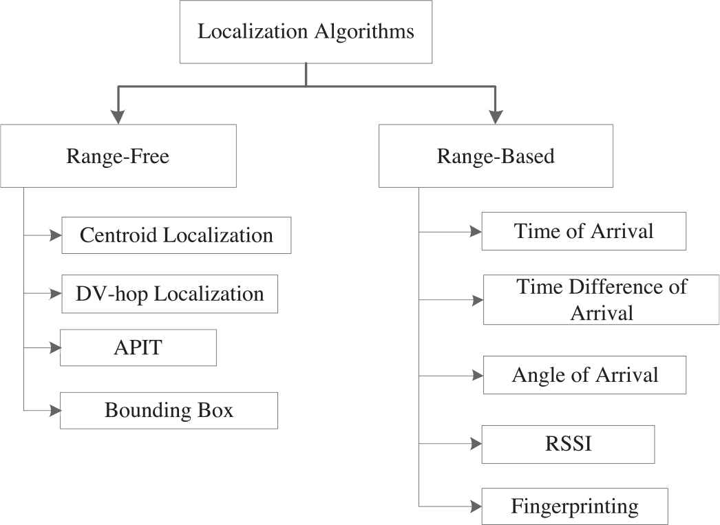
Classification of localization algorithms.
The main parameter used by range-based localization methods in location determination is distance.
Time of arrival (TOA): When the propagation velocity of the signal between transmitter and receiver nodes and the time lapsed during transmitting the signal is known, and then the distance is calculated using Equation 1.
Time difference of arrival (TDOA): This is a method used for eliminating the time synchronization problem in TOA [9]. The basic logic of the method is to use two separate signals with different propagation velocities. For example, let the transmitter node send a radio signal at time t1 and let the signal reach the receiver at time t2. We assume that the sound (as the second signal) is sent at time t3 = t1 + twait and reaches the receiver at time t4. The distance between the transmitter and receiver is calculated by using these two signals, as shown in Equation 2.
The disadvantages of this method are the need for two separate signal generators for two separate signals and its high cost.
Received Signal Strength Indicator (RSSI): This is a value that indicates the incoming signal strength in dBm. As the signal strength decreases, the dBm value of RSSI decreases. The small RSSI value means that the distance will be large. Because the RSSI value can easily be calculated in many communication chips, there is no need for additional hardware. Thus, location determination with RSSI is an economical method [10].
Angle of arrival (AOA): Location determination with this method is performed according to the incoming signal angle in an open and free-space environment where wireless sensor nodes “see” each other directly [11]. Because additional equipment, such as a dish and a microphone, must be used for detecting the incoming signal angle, this method has high cost and accuracy in location determination.
Range-free methods are hardware-independent, and therefore are cost-effective. However, their error rates in location determination are higher than for range-based methods. Instead of distance, these methods aim to determine the location by using different parameters, such as hop count.
Distance vector-hop (DV-HOP): The anchor nodes with known location information transmit a data package with a counter variable, whose location information and initial value is 0, to other anchor nodes by means of neighbor nodes on the network. When data packages are transmitted to each node on the network, the counter value in the data package is incremented by one. When data packages reach the anchor node in different ways, the average jump distance is calculated according to the data package with the smallest anchor node counter value [12].
Approximate point in triangle (APIT): Three anchor nodes are selected each time from N anchor nodes, and testing is done to determine whether the searched node is in the triangle formed by these three anchor nodes. After this operation is performed for all anchor nodes, the searched node is assumed to be at the intersection of these triangles [13].
Centroid: This is a method with a high error rate that locates the free sensor node to the intersection point of at least three anchor nodes. It is the simplest one among all location determination methods [14].
Bounding box method: In this algorithm, after finding the estimated distance to the anchor nodes, quadratic areas are generated around the anchor nodes according to this distance information. The node, whose location is to be determined, is assumed to be at the intersection area of quadratic areas. The estimated location is the center of the area formed by the intersection [15].
1.1. Motivation
Location determination methods require RSSI and distance measurements. Measuring both parameters causes large errors in location determination. The main purpose of this article is to develop a cascade artificial neural network (ANN)-based fingerprint location determination method that uses only RSSI measurements to perform location determination. A mobile device was designed for implementing the proposed algorithm. Also in this article, the location of the mobile device has been determined with minimum error by entering the RSSI values measured by means of the mobile device to the algorithm.
1.2. Our Contributions
The main contributions of this paper are listed as follows:
A mobile device has been developed that can move very precisely, operate in real time, and make an Radio Frequency (RF) communication.
In a 15.6 × 13.8 m2 environment, a fingerprint step has been selected as 60 cm. A Cascade ANN-based fingerprinting algorithm has been developed to determine the location of the mobile device in this environment.
The proposed system performs the location determination with minimum error because it uses only RSSI signals.
According to the results obtained, the maximum error is 0.91 m, the minimum error is 0.013 m, and the average error is 0.248 m. When comparing the results with those in the literature, it has been revealed that the location error has been significantly decreased.
1.3. Structure of the Paper
The rest of this paper is organized as follows. In Section 2, the studies in the literature are summarized. In Section 3, the conventional fingerprint localization algorithm is given. In Section 4, the design and structure of the linearly moving mobile device is explained. In Section 5, the implementation environment, the structure and programming of the anchor node used, and the offline and online processes of the proposed algorithm are explained in detail. In Section 6, the findings obtained from real-time tests and the evaluation of the results is presented. Finally, conclusions are drawn in Section 7.
2. RELATED WORKS
Considering the disadvantages of GPSs, the use of range-free localization algorithms is a cost-effective approach for indoor environments. However, the main limitations of this approach are estimation precision, node density, sensing coverage, and topology diversity. Comprehensive research has been done on wireless localization based on soft computing techniques over the last decade to overcome these problems. Pau et al. suggested the fuzzy logic controller (FLC) for location determination. They used the particle swarm optimization (PSO) technique to minimize the location error and obtain the optimal configuration of the FLC by processing the data obtained from the anchor nodes. The membership functions of the FLC were optimized with the help of PSO, and location error was reduced to minimum levels [16]. Amri et al. proposed a new algorithm for geographic routing. The location determination in their proposed mechanism was based on fuzzy logic and WCL. They used Sugeno and Mamdani–type fuzzy systems to determine the sensor location accurately and to increase the accuracy of the WCL algorithm. With the Mamdani-based localization method, the maximum location error was calculated as 1.20 m while, the minimum location error was 0.15 m. In the Sugeno-based fuzzy logic system, the maximum and minimum values were calculated as 0.85 and 0.05 m, respectively. The average location errors obtained were 0.8 and 0.3 m for Mamdani and Sugeno, respectively [17]. Phoemphon et al. suggested a soft computing-based hybrid structure to develop a centroid localization algorithm (CLA), a range-free-based localization. In the suggested method, the fuzzy logic system was integrated into the CLA. An extreme learning machine optimization technique was used by utilizing the strengths of the fuzzy logic and CLA [18]. Tuncer et al. proposed a fuzzy and genetic algorithm (GA)-based structure to determine the location of a mobile sensor in a closed environment. The proposed method converts the CLA to the intelligent centroid localization (ICL) algorithm. The RSSI values measured with the anchor nodes were applied as input to the fuzzy system in the developed ICL. Fuzzy system membership functions were set using the GA to minimize location errors. The results were compared with the centroid and APIT algorithms. Location error was reduced by 57% and 65% compared to the centroid and APIT algorithms, respectively [19]. Egger et al., with the help of the AOA estimation algorithm, presented a GA approach to select the relevant radar design parameters. First, they performed a simulator that could evaluate the localization performance with a set of specific design parameters. The simulator output was used as a part of the GA objective function investigating the range of solutions for optimal design parameters. By means of this approach, the quadratic error obtained by the radar design using the parameters selected by a human was decreased by half with the proposed localization algorithm [20]. Gholami et al. proposed an ANN-based structure to minimize location error in real environments. Network performance was examined by considering different noise and signal attenuation sources in the real world. In a 200 × 300 m2 test area, the location of a mobile node was determined at a 95% confidence interval. The accuracy and effectiveness of the results obtained were compared to those of the trilateration algorithm, and successful results were obtained [21]. Tuncer et al. developed an ANN model to determine the location of a mobile phone in an indoor environment. The ANN model accepts the RSSI values measured by the mobile phone from three anchor sensors, as well as the anchor sensor ID number as the input. First, the ANN was trained and then tested. Errors obtained from the tests were determined by comparison of the locations of a mobile phone and the actual locations. The results were compared with the CLA method in the literature and the location error was reduced by up to 70% [22].
In addition to the soft computing and range-free localization algorithms briefly summarized above, there are also studies applying soft computing to the fingerprint algorithm [23, 29]. Orujov et al., with Bluetooth technology, conducted an experimental study of indoor localization algorithms based on RSSI. Proximity, centroid, weighted centroid, weighted-compensated, WCL based on RSSI, fingerprint, and trilateration localization algorithms were applied and then compared. A fuzzy logic-based schema was proposed and evaluated in real-world conditions to determine the optimal algorithm for the indoor environment. Experimental results showed that the fingerprint localization algorithm was optimal and the location error was 0.67 m [23]. Hernandes et al. proposed a model with a fingerprint approach using Wi-Fi. A Hierarchical Localization and Fuzzy Classifier-based model was tested under real conditions in an indoor environment. The average error was decreased by 55% compared to conventional fingerprint localization [24]. Oussalah et al. examined the fingerprint problem for location determination in closed environments based on RSS measurements. In the fuzzy logic-based approach, the localization of the target node was determined as a weighted combination of the nearest fingerprints. The weights obtained were given as an input to the Tagaki-Sugeno Fuzzy controller. A 20 × 20 m2 area was used for the implementation, the distance between two fingerprints was selected as 1.5 m, and the location error was reduced [25]. Khatab et al. developed a Fuzzy Least Squares Support Vector Machine-based indoor fingerprint system by using RSS. The average estimation error of the proposed system was 2.56 m [26]. Ngo et al. proposed a two-phase structure to improve the performance of the fingerprint algorithm. The first phase was to minimize the changes in the RSS, while the second phase was to measure the distance. Numerical results showed that their system performed well in terms of accuracy and reliability [27]. Subedi et al. performed a localization determination by combining conventional fingerprint localization and WCL methods. The number of reference points (RPs) was decreased in the suggested method. The system was performed in two steps: In the first step, a fingerprint algorithm was performed by using RP and WCL. By using the estimated location in the first step, the actual location was determined in the second step by rerunning the WCL algorithm. The location error was decreased more than 40% [28]. Zhang et al. proposed an RSSI-based Fingerprint Feature Vector algorithm. The location area was divided into grids, and location accuracy was provided by means of similarity matching between a real-time RSSI feature and an RSSI fingerprint database feature based on vectors of mobile devices [29].
3. FINGERPRINT LOCALIZATION ALGORITHM
Wi-Fi-based fingerprint localization technology is one of the most popular localization technologies based on 2D modeling [30, 31]. Fingerprint localization technology mainly uses the signal as the fingerprint step which is stored in the database. The signal strength received from each location is obtained by matching the signal strength measured in the locations of the users for location determination. In the fingerprint technique, first the closed area is divided into grids, whose coordinates are known, and then RSSI values obtained from all the anchor nodes for each grid are saved in a database. The RSSI map is created at this phase. Figure 2 shows the RSSI obtained from the anchor nodes and the storage of locations in the database. Secondly, RSSIs obtained from any location are given as inputs to the localization algorithm. The result obtained from the algorithm output is the sensor location.
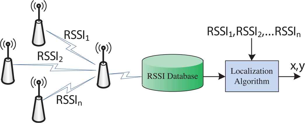
A scheme for fingerprint algorithm.
When compared to other localization systems, fingerprint localization technology has the advantages of low cost and high precision. This algorithm is ideal for modeling the environment without requiring determination of the exact location of the anchor nodes. The locating accuracy of this method is greater than for other localization algorithms. Fingerprint localization technology requires different algorithms; therefore, its computational consumption and algorithm complexity is relatively high. In addition, because the fingerprint algorithm requires a large amount of preliminary information, the preliminary study has a high cost factor. After the anchor location or internal environment is changed, it is necessary to retrieve the RSSI data and remodel the media.
In the fingerprint algorithm, data collection and recording is the first phase, which is called the offline process. The main task at this phase is to collect fingerprint data. The second phase of the fingerprint algorithm is known as the online process. In the online phase, a model is created for location determination. With this model, location determination is performed by using the database created in the offline phase.
There are two main methods to collect fingerprint data: correct modeling and empirical modeling. In the empirical modeling used in this article, the signal strength taken from the anchor nodes placed in different coordinates is measured in the location to be determined. Fingerprint data, also called signal strength, radio map, or database, is stored with the anchor node locations and other information (such as Media Access Control (MAC) address). Because empirical modeling is based on many data samples, the workload in the initial phases may be large. This modeling method depends on an indoor environment; however, it has a high level of accuracy.
4. DESIGN OF A LINEARLY MOVING MOBILE DEVICE
It is necessary to create a fingerprint database for location determination with the suggested method. A mobile device was needed in this study. The mobile device we have developed has precise movement capability, and it can perform RF communication with the anchor nodes. Considering the need for a sensitive, moving structure in our selection of the equipment to create the mobile device, the mDrawbot kit (from the Makeblock company), which includes a stepper motor, was selected [32]. The device is equipped with two stepper motors, two wheels, one caster wheel, two motor-drive cards, one control card, two series power units of 5 V and 5200 mAh, and one XBee module to control the device via a computer.
The main task of the mobile device we developed is to move to different grid points and communicate with the anchor nodes in the implementation area. By means of the signals transmitted by the mobile device to the anchor nodes, the anchor nodes should be able to measure the signal strength to be used for location determination.
One of the most important points to be considered in designing the device is that the center of gravity should be on the vertical axis of the device. If the center of gravity were not on the vertical axis, this could cause the device to deviate to the right or left. This is a matter that can cause errors in creating a fingerprint database. Tests were performed on each grid point of the device for its straight movement, and extra weights were added to some points to the device. To supply the energy of the device (to drive the stepper motors and the XBee module), two power banks with 5 V power output were connected in series, and a 10 V voltage was obtained. The XBee module, which is used to enable the device to communicate with a PC, operates with a 3.3 V supply. Because there was no 3.3 V voltage output in the device control circuit, a 3.3 V voltage was obtained by using an appropriate regulator to feed the XBee module.
The stepper motors used in the new mobile device are those with 200 steps. This means that the rotor will perform a full rotation in 200 steps. That is, the number of steps required for a 360-degree rotation of the rotor is 200. Therefore, each step has a rotation angle of 1.8 degrees. In order to increase the sensitivity of the device, the micro step mode was selected as 1/16 step on the motor driver board. Accordingly, the step number of the stepper motor having 200 steps was found to be 200 * 16 = 3200, and the sensitivity was increased. To move the device from one grid point to another one, it is necessary to calculate the number of steps that stepper motors will take. The first thing to know is the wheel circumference, which is 20.3 cm for the mobile device. How to determine the step number of the stepper motor for a particular distance on a flat surface is shown in Equations 3 and 4.
For example, for wc = 20.3 and x = 60 cm; n = (3200*60)/20.3 = 9456,
where wc is the wheel circumference in cm, xs is the distance covered by one step, n is the number of steps, and x is the distance covered by the device. In the application, the distance between grid points was determined to be 60 cm. For the movement of the mobile device from one grid point to another one, the number of steps was calculated as 9456 by using Equations 3 and 4. A general view of the new mobile vehicle is shown Figure 3.
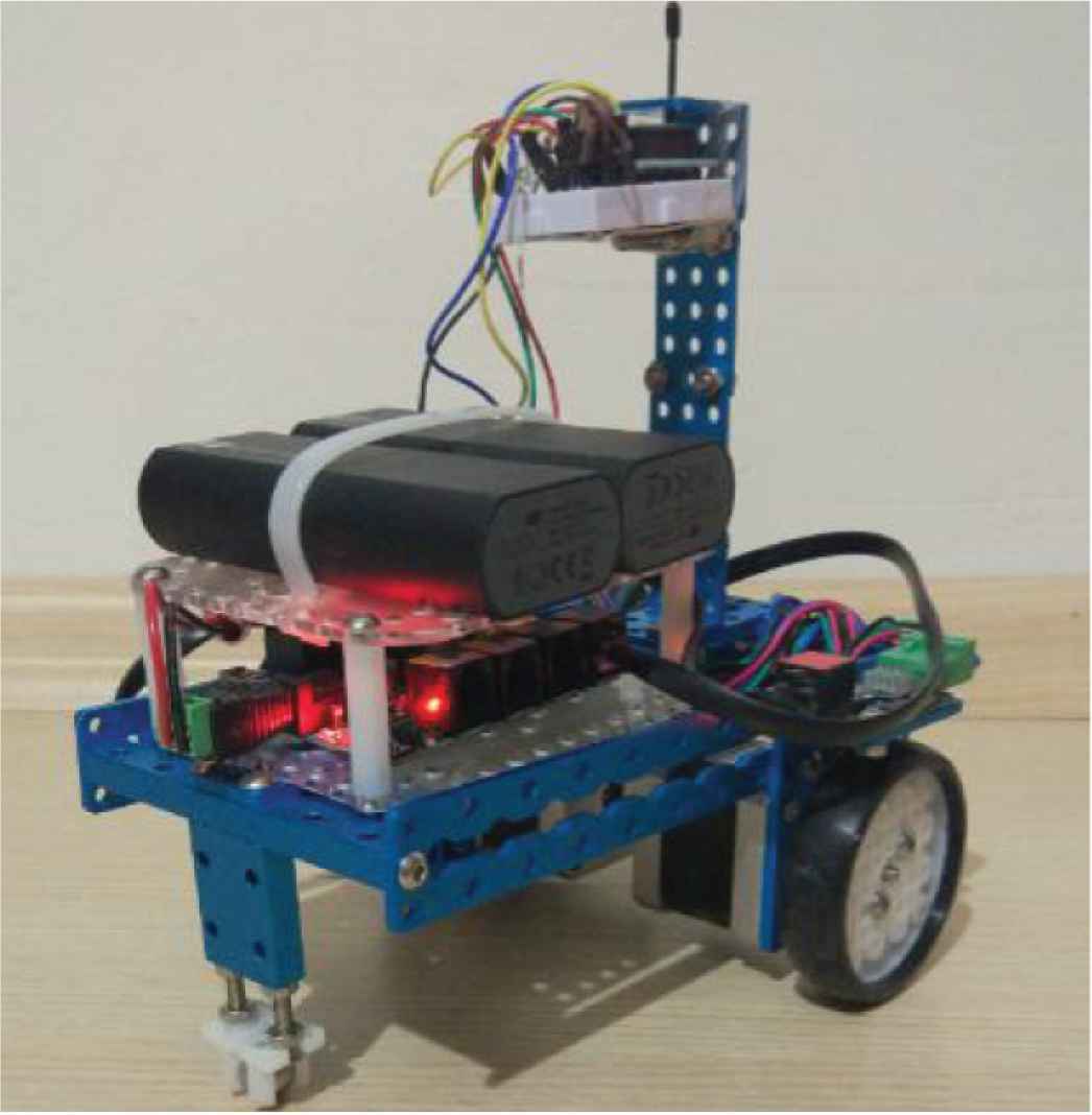
General view of the mobile device.
5. PROPOSED SYSTEM ARCHITECTURE
In this article, a 15.6 × 13.8 m2 implementation area was selected for the location determination with the proposed cascade ANN-based fingerprint localization algorithm. This environment is a flat surface in a real-world environment, namely, the load dispatching main control room of the technical building of EÜAŞ Keban HES Management Directorate. Because the ground of the room was floored with 60 × 60 cm tiles, the fingerprint step of the mobile device to be designed was selected as 60 cm. Figure 4(a) shows the coordinate system of the implementation area, while Figure 4(b) shows the real environment and mobile device.
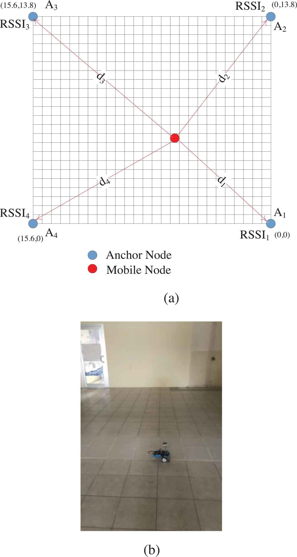
(a) Anchor nodes and coordinate system. (b) Real implementation environment and mobile device.
In this selected area, a two-phase process was carried out to perform the location determination system, involving offline and online processes. A1, A2, A3, and A4 anchor nodes were placed at each corner of the implementation area. In these nodes, Xbee modules (Digi Company) were used as Zigbee communication module [33]. As shown in Figure 4(a), three XBee modules (A2, A3, and A4) were used as the corner nodes, one module was used as the base station (A1), and the remaining XBee module was used in the mobile device.
In the offline process, the A1 base station stores the RSSI values obtained from anchor nodes and real location information in a database. The definition of the data that is saved in the database in the offline process is as follows.
This work represents database using the set DB, which contains the n generated fingerprints. Each element of DB is defined as a tuple. The index i identifies the fingerprint in the database.
The set Ri is the measurement data set collected during the offline phase at the coordinates Ci. Di is a set of distances to the anchor nodes of the coordinates.
The A1 base station communicates with both the environment and the PC, where the data is stored in the database. After creating the fingerprint database, the online process is executed. The most important problem at this phase is to develop a model that can predict the location determination with minimum error. The signal strength (RSSI values) between the anchor node and the mobile device with unknown location is measured by anchor nodes to determine the location of a mobile device in any location. Measured RSSI values are given as the input to the proposed algorithm and the location is determined. The cascade ANN model was proposed in this article for offline and online processes. The basic structure of the proposed system is shown in Figure 5.
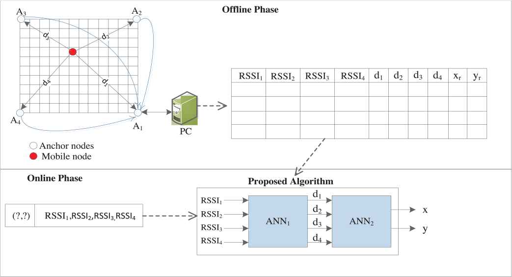
Proposed cascade artificial neural network (ANN)-based fingerprint algorithm.
5.1. Experimental and Hardware Implementation
An Arduino Uno electronic card was selected because of the ease of programming of nodes A1, A2, A3, and A4 as an electronic control board and because of its rich library support. Thanks to these cards, the data coming to XBee modules can be read, and similarly the data can be transmitted through XBee modules to another XBee module via serial communication. The main task of these nodes, consisting of the Arduino Uno, the XBee module, and an appropriate power supply is to calculate the RSSI value of the signal coming from the XBee module in the mobile device and then to transmit it to the base station A1 node. The XBee modules used in the corner nodes, as in all the XBee modules used in the application, were set by Digi Company’s XCTU configuration software tool so that the Application Programming Interface (API) mode was active and the API output mode was “native.” The purpose of these adjustments is to transmit data packages coming to the XBee modules directly to the Arduino control card via the Universal Asynchronous Receiver-Transmitter (UART) serial port. When a data package is transmitted to the Arduino via the UART, the Arduino commands the XBee module to calculate the RSSI value by sending a “DB” AT command. The XBee module fulfills the requirements of this command and transmits the calculated RSSI value to the Arduino. The Arduino creates a data package, including the RSSI value as the data and also including the address of the Base Station A1 corner node, and then transmits this data package to the XBee module of A1. Therefore, the RSSI values can then be transmitted to the PC via the base station node. Three corner nodes performing these tasks were formed and placed in the corners of the room selected as the study area. Figure 6 shows one of the corner nodes consisting of a 5 V power supply, the Arduino, and the XBee module.
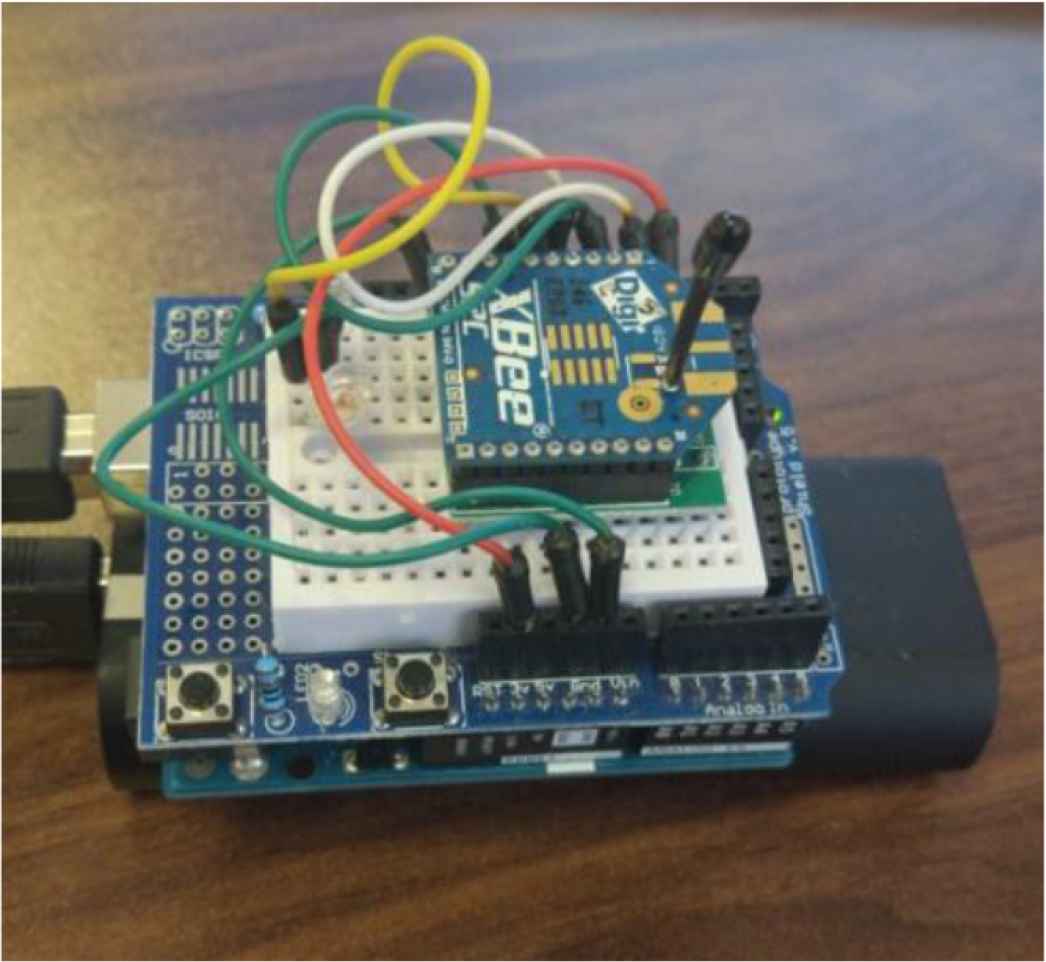
General view of anchor nodes.
5.2. Program Structure for Anchor Node A1
The base station called A1 is connected to a computer via the USB port, as shown in Figure 5. The data coming to this node is transmitted to the computer via the USB port. Similarly, the data transmitted from the computer to the XBee module on node A1 can be transmitted to other anchor nodes. The main tasks of this node are to transmit commands to the mobile device, calculate the RSSI values of the signals coming from the device, and transmit the RSSI values coming from the A2, A3, and A4 nodes to the computer. It is shown in Figure 5 that the RSSI values calculated by the anchor nodes, which are the data packages sent by the mobile device in any coordinate, are recorded in the database via the anchor A1.
The XBee module, which is used for both remote control of the device with the PC and communication with the anchor nodes, is connected in series with the UART pins on the 5th port of the Ardunio Uno control card. The main task of the device is to communicate with the anchor nodes according to the commands sent from the computer to the Xbee module of the device and to move in the x-axis. For the linear movement of the device on the ground, the commands “a,” “b,” “c,” “d,” and “e” can be taken from the PC. When the command “a” transmitted by the PC and base station is given to the mobile device, the device sends a data package with insignificant content to A1 through the XBee module. Similarly, an insignificant data package is sent to A2, A3, and A4 for “b,” “c,” and “d” commands, respectively. The aim is to achieve the calculated signal strength (RSSI) between the node and device. The anchor nodes receiving the command then measure the signals RSSI1, RSSI2, RSSI3, RSSI4, and transmit them to the base station. When the last command, “e” is transmitted to the mobile device, the device moves by 60 cm. Thus, the implementation area divided into grids can be scanned.
5.3. Offline Process
In the offline phase of the proposed system, when the mobile device is at point (0, 0), the computer is commanded to send an insignificant data package to the A2 anchor node through the base station’s A1 node. When the data arrives from the device at the A2 anchor node, the RSSI value is calculated on this node and transmitted to the base station A1 anchor node, which is connected to the computer. The RSSI value coming to the A1 node is transmitted to the computer and stored through the program, which is running on the computer. These steps are repeated 100 times for each anchor node, including the base station. In total, 400 RSSI values are obtained for each point. The average RSSI value for each anchor node and the actual device location and distances are saved in the MySQL database. Then, the command “move by 60 cm” (command e) is sent to the mobile device from the computer, and the device is moved to its next location. This process is repeated for all points. As a result, when the mobile device has traveled from point (0, 0) to point (15.6, 13.8), a total of 26 × 23 × 100 = 59,800 RSSI values are obtained for each anchor node. When averaging the RSSI for each anchor node, the number of values recorded in the database becomes 26 × 23, that is, 598. Figure 7 illustrates the flowchart required to perform the offline process.
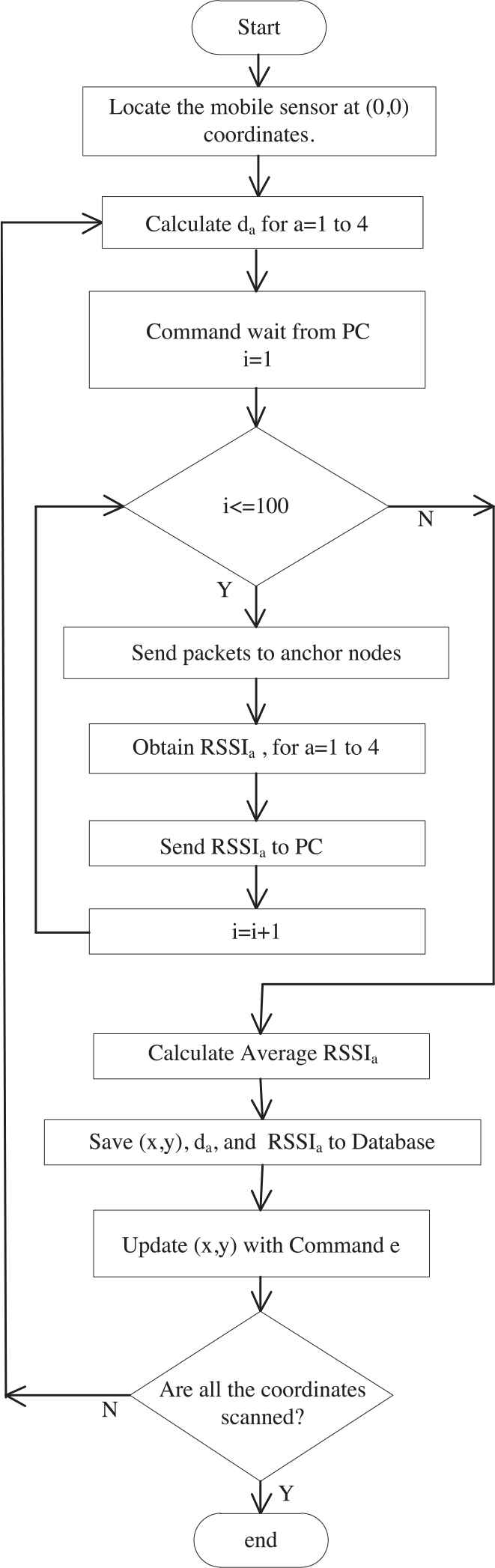
Offline process flowchart.
Step 1: Calculate the distances between the coordinate of the device to the anchor nodes.
da is the distance between the anchor node and mobile device, (xa, ya) are the coordinates of the anchor node, and (xm, ym) are the coordinates of the mobile device. The distance between the mobile device and the anchor node is calculated according to Equation 5.
For example, if the mobile device is at the xa = 1.8, ya = 2.4 coordinate, its distance to A1 (xa = 0, ya = 0) node is calculated as 3 cm. The distances (d2, d3, d4) to other anchor nodes (A2, A3, A4) are calculated in a similar way.
Step 2: Wait for a command from the base station.
Step 3: Send a blank data package to the anchor nodes according to the type of command (a, b, c, and d).
Step 4: Measure RSSI value of anchor nodes for each data package and transmit RSSIs to the A1 anchor node.
Step 5: Send RSSI1, RSSI2, RSSI3, and RSSI4 values obtained at the A1 node to the PC.
Step 6: Calculate the average of 100 RSSI values coming from each anchor node in the PC.
Step 7: Record the average RSSIs, location (xr, yr), and distances (d1, d2, d3, d4) to the database.
Step 8: Move to the next coordinate with the command e.
Step 9: If all coordinates are not scanned, go to Step 1.
Step 10: Database was created.
A software program was developed using the JAVA programming language to perform the tasks (transmit a command, collect RSSIs, etc.) that the A1 anchor node should do. Figure 8 shows the data package coming to the A1 anchor node and the RSSI value measured by the A1 node. When the mobile device is at the (0.6, 0.6) coordinate, the data package content is “72 73 73 69,” as shown in Figure 8 (this value is the ASCII equivalent of RSSI characters), and the RSSI value measured by the A1 anchor node is −53.
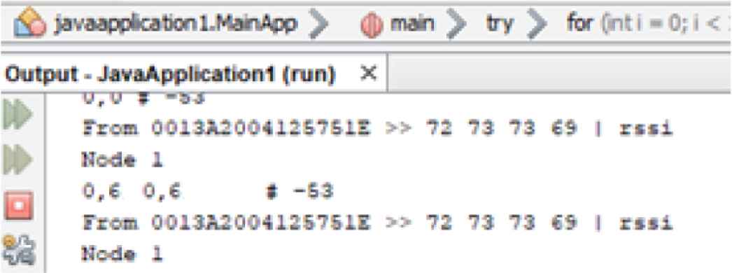
Measurement of received signal strength indicator (RSSI) value.
Thus, the training data for the cascade ANN-based fingerprint localization algorithm were obtained. The RSSIs saved in the database are given to the cascade ANN model as the input, thus performing the training. ANN1, as shown in Figure 9, has 3 layers, for which the inputs are RSSI1, RSSI2, RSSI3, RSSI4, and the outputs are d1, d2, d3, d4. There is also a hidden layer. The training algorithm used at this phase is Levenberg–Marquardt and the error is trained using all records in the database until it is less than 0.01. The ANN2 model is also 3-layered, and the first layer inputs are d1, d2, d3, and d4, which are the trained outputs of ANN1. The output layer of ANN2 is the coordinate value of each grid point in the database (xr, yr). The Levenberg–Marquardt algorithm was used in training ANN2. The training was continued until reaching a 0.01 error. The online process was initiated after training both ANN models.
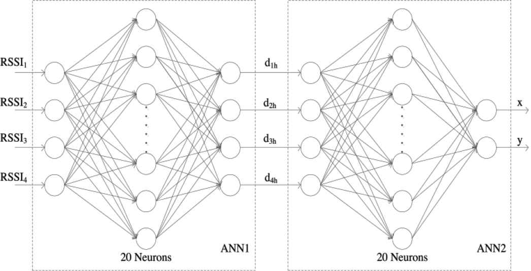
Cascade artificial neural network (ANN) structure.
5.4. Online Process
When the mobile device was in any location, the RSSI values measured on the anchor nodes were given as inputs to the trained cascade ANN model. Firstly, the distance of the mobile device to the anchor nodes was calculated by ANN1. The distances obtained from ANN1 were given as input to ANN2, and the location of the mobile device was obtained. For example, when the mobile robot was at the (0.31, 8.08) coordinate, the measured RSSI values were −91.88, −125.85, −121.39, and −75.80. When these RSSI values were given as the input to ANN1, the distances obtained were 8.29, 17.29, 16.32, and 5.73 m, respectively. When these distance values were given as inputs to the ANN2 model, the location of the mobile device (0.68, 8.22) was obtained. By using the actual location of this mobile device (0.31, 8.08) and the location estimated from the cascade ANN algorithm (0.68, 8.22), the distance between two points (location error) was found to be 0.39 m, with the help of Equation 5.
6. EXPERIMENTAL RESULTS
6.1. Finding
For testing the cascade ANN-based fingerprint algorithm with the help of data obtained from the implementation environment divided into 60 cm grids, 100 sample coordinates with unknown locations were randomly selected. The location estimation of the mobile device positioned in these coordinates was determined with the help of the proposed algorithm with minimum error. Figure 10 shows the actual location and estimated locations of the mobile device.
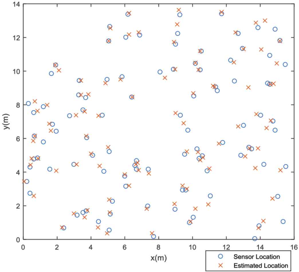
Real sensor locations and estimated locations.
RSSI1, RSSI2, RSSI3, and RSSI4 values measured at these coordinates were given as input to ANN1. Table 1 shows randomly obtained actual coordinates (xr, yr) in meters and some samples of RSSI values measured at these coordinates.
| Sample No. | xr | yr | RSSI1 | RSSI2 | RSSI3 | RSSI4 |
|---|---|---|---|---|---|---|
| 1 | 0.31 | 8.08 | −91.88 | −125.85 | −121.39 | −75.80 |
| 2 | 12.47 | 9.41 | −121.77 | −99.36 | −73.32 | −114.91 |
| 3 | 4.65 | 7.38 | −93.82 | −114.32 | −112.46 | −89.78 |
| 4 | 2.73 | 7.35 | −90.49 | −116.86 | −115.67 | −85.64 |
| 5 | 3.31 | 9.44 | −101.63 | −122.45 | −114.23 | −74.55 |
| 6 | 6.06 | 3.17 | −84.82 | −100.23 | −117.49 | −109.55 |
| 7 | 8.97 | 1.80 | −97.05 | −85.01 | −116.36 | −117.99 |
| 8 | 4.44 | 1.05 | −65.84 | −105.19 | −125.35 | −114.10 |
| 9 | 6.07 | 12.01 | −114.15 | −120.91 | −99.07 | −81.20 |
| 76 | 10.17 | 10.47 | −118.21 | −107.30 | −80.53 | −102.74 |
Measured received signal strength indicator (RSSI) values.
The estimated distances obtained at the output of ANN1 were given as the input to ANN2. The distances of randomly taken mobile device locations to anchor nodes d1h, d2h, d3h, and d4h were calculated at the output of ANN1 in m. Figure 11 shows the absolute errors of the distances obtained for 100 randomly taken coordinate points (Errdi = abs(di- dih)). The average values of the distance errors Errd1, Errd2, Errd3, and Errd4 are 0.126, 0.136, 0.131, and 0.159 m, respectively. It is seen that absolute errors and their average values are close to each other for all distances. Table 2 shows actual distances (di), calculated distances (dih), and absolute errors (Errdi).
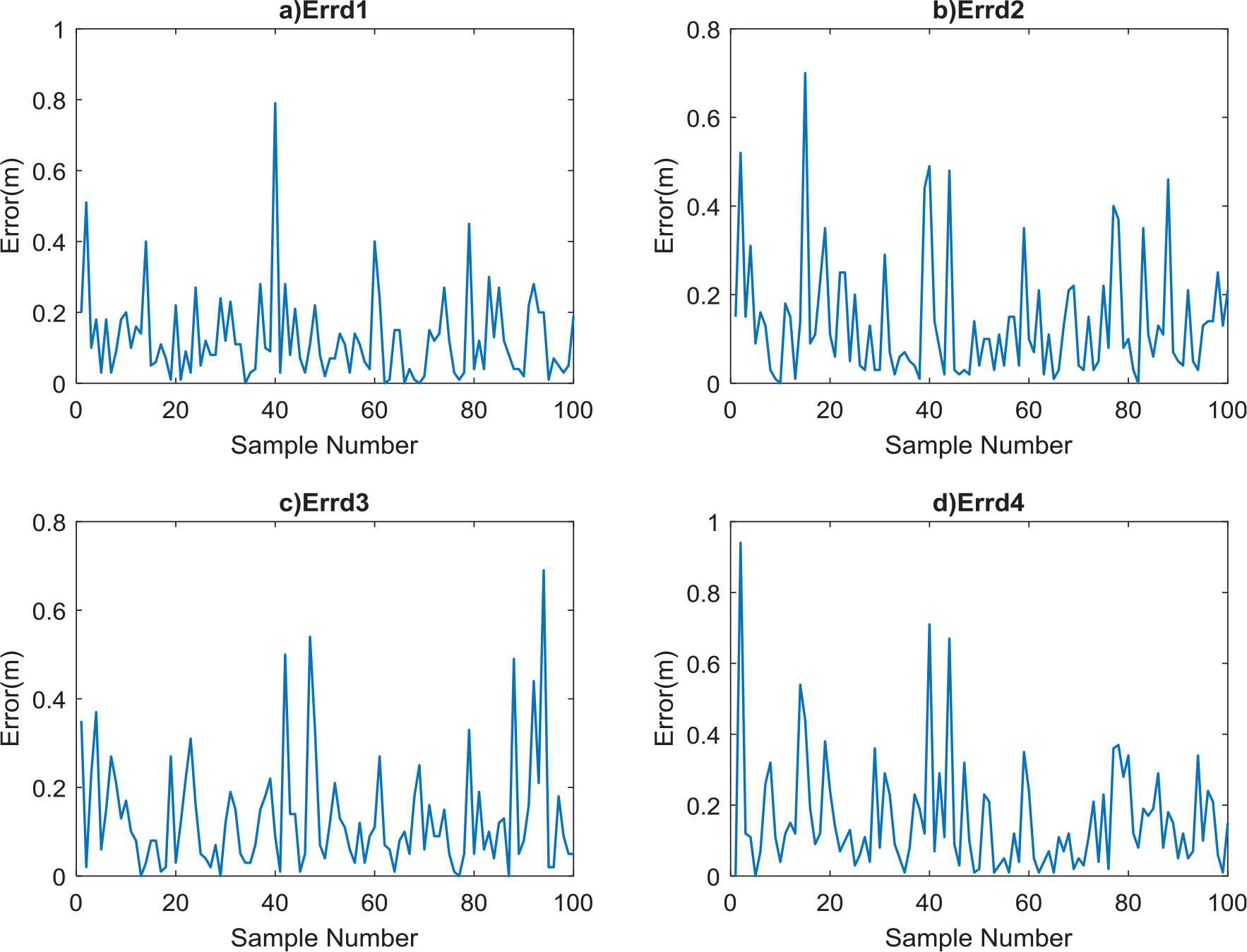
Errd1, Errd2, Errd3, and Errd4 variations.
Sample No. | d1 | d1h | Errd1 | d2 | d2h | Errd2 | d3 | d3h | Errd3 | d4 | d4h | Errd4 |
|---|---|---|---|---|---|---|---|---|---|---|---|---|
| 1 | 8.08 | 8.29 | 0.20 | 17.29 | 17.14 | 0.15 | 16.32 | 15.98 | 0.35 | 5.73 | 5.73 | 0.00 |
| 2 | 15.62 | 16.13 | 0.51 | 9.91 | 9.40 | 0.52 | 5.40 | 5.38 | 0.02 | 13.22 | 14.16 | 0.94 |
| 3 | 8.73 | 8.63 | 0.10 | 13.21 | 13.36 | 0.15 | 12.69 | 12.92 | 0.23 | 7.92 | 7.81 | 0.12 |
| 4 | 7.83 | 8.01 | 0.18 | 14.82 | 14.51 | 0.31 | 14.40 | 14.03 | 0.37 | 7.01 | 7.11 | 0.11 |
| 5 | 10.01 | 9.98 | 0.03 | 15.50 | 15.41 | 0.09 | 13.04 | 12.98 | 0.06 | 5.47 | 5.47 | 0.00 |
| 6 | 6.83 | 7.02 | 0.18 | 10.06 | 9.89 | 0.16 | 14.29 | 14.13 | 0.15 | 12.24 | 12.30 | 0.07 |
| 7 | 9.15 | 9.12 | 0.03 | 6.87 | 6.99 | 0.13 | 13.70 | 13.43 | 0.27 | 14.98 | 14.72 | 0.26 |
| 8 | 4.57 | 4.48 | 0.09 | 11.21 | 11.17 | 0.03 | 16.94 | 17.15 | 0.21 | 13.50 | 13.82 | 0.32 |
| 9 | 13.46 | 13.64 | 0.18 | 15.33 | 15.32 | 0.01 | 9.69 | 9.56 | 0.13 | 6.33 | 6.44 | 0.11 |
| 76 | 14.60 | 14.63 | 0.03 | 11.79 | 11.88 | 0.11 | 6.37 | 6.38 | 0.01 | 10.70 | 10.72 | 0.02 |
Distances of randomly obtained mobile device locations to anchor nodes and errors.
Figure 12 shows the variation of the location errors obtained for 100 samples. According to the results obtained, the maximum error (0.91 m) was obtained in the second sample, while the minimum error (0.013 m) was obtained in the 76th sample, as shown in Table 3. The term n indicates the number of samples. The estimated coordinates and the average error of the errors between actual locations (Err) are given according to Equation 6.
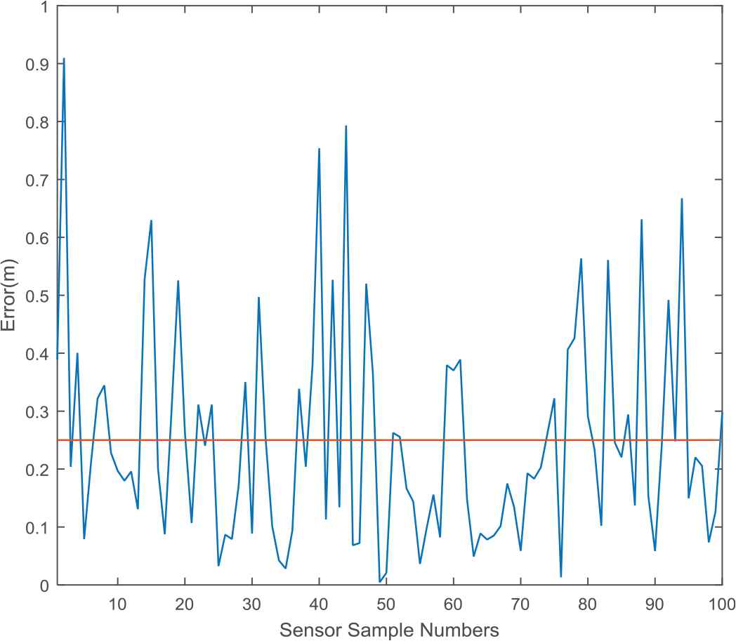
Location error variations.
For 100 different coordinates of the mobile device, the average error of the locations obtained from the algorithm was found to be 0.248 m using Equation 6. Among 100 different locations, the error was lower than the average error for 61 locations, while it was higher than the average error for 39 locations. The average error calculated as 0.248 is plotted as a line in Figure 12. Table 3 shows the actual locations (xr, yr), the calculated locations (xh, yh), and the location errors (Err) in m.
| Sample No. | xr | yr | xh | yh | Err |
|---|---|---|---|---|---|
| 1 | 0.31 | 8.08 | 0.68 | 8.22 | 0.39 |
| 2 | 12.47 | 9.41 | 13.30 | 9.03 | 0.91 |
| 3 | 4.65 | 7.38 | 4.45 | 7.35 | 0.20 |
| 4 | 2.73 | 7.35 | 3.13 | 7.37 | 0.40 |
| 5 | 3.31 | 9.44 | 3.39 | 9.43 | 0.08 |
| 6 | 6.06 | 3.17 | 6.26 | 3.20 | 0.21 |
| 7 | 8.97 | 1.80 | 8.93 | 2.12 | 0.32 |
| 8 | 4.44 | 1.05 | 4.40 | 0.71 | 0.34 |
| 9 | 6.07 | 12.01 | 6.25 | 12.16 | 0.23 |
| 76 | 10.17 | 10.47 | 10.17 | 10.48 | 0.013 |
Real locations, calculated locations, and location errors.
| Ref. No. | Algorithm | Max. Error | Min. Error | Ave. Error |
|---|---|---|---|---|
| [17] | Mamdani fuzzy–based localization Sugeno fuzzy–based localization | 1.20 0.85 | 0.15 0.05 | 0.5 0.3 |
| [34] | Mamdani fuzzy–based localization Sugeno fuzzy–based localization | 2.02 2.01 | 0 0 | 0.89 0.94 |
| [35] | Mamdani fuzzy–based localization Sugeno fuzzy–based localization | 2.01 1.96 | 0.12 0.14 | 0.89 0.94 |
| [19] | Centroid based on fuzzy logic and genetic algorithm | − | − | 0.98 |
| [22] | Artificial neural network (ANN)-based localization | − | − | 0.88 |
| [23] | Fuzzy-based localization | − | − | 0.67 |
| [24] | Hierarchical classifier ensemble | − | − | 1.22 |
| [26] | Fuzzy Support Vector Machine–based fingerprint | − | − | 2.56 |
| [27] | Variance reduction (VR)–based fingerprint distance metric learning + VR-based fingerprint Multiple discriminant analysis–based fingerprint Kernel Support Vector Machine–based fingerprint | − | − | 0.71 0.61 0.68 0.69 |
| [28] | Weighted centroid localization fingerprint | 1.14 | 0.867 | − |
| [36] | Adaptive K-nearest–based fingerprint | − | − | 1.0 |
| Proposed | Cascade ANN–based fingerprinting | 0.91 | 0.013 | 0.248 |
Comparison of the proposed system with the literature.
6.2. Evaluation
Table 4 presents a comparison of the proposed system with soft computing algorithms. As shown in Table 4, the minimum values are found in ref. [17]. According to the results obtained in this reference, the minimum, maximum, and average location errors are 0.85, 0.05, and 0.3 m, respectively. The maximum, minimum, and average errors obtained with the proposed algorithm were measured as 0.91, 0.013, and 0.248 m, respectively. When the proposed method is compared with ref. [17], it is seen that our average and minimum errors are smaller by 17% and 75%, while the maximum error is higher by 7%. The fingerprint step taken in this article was selected to be smaller than others in the literature, and errors were reduced to minimum levels. The environment was divided into 1.25 × 0.9 m2 grids with the fingerprint step selected from ref. [28]. The minimum and maximum errors obtained were 0.867 and 1.14 m, respectively, as seen in Table 4. In the proposed method, the selected fingerprint step was divided into grids of 0.6 × 0.6 m2. Thus, it was seen that the location was determined with a lower error than in the literature. According to the results, the proposed algorithm was better than the fingerprint algorithms in the literature. The main reason for the low error is the precision of the mobile device design and the small fingerprint step.
7. CONCLUSION
Fingerprint-based localization is a time-consuming algorithm that requires too much effort for efficient utilization. Moreover, a large amount of data must be collected from the environment to create a fingerprint database. Despite these disadvantages, it is an algorithm with high accuracy. In this paper, a cascade ANN-based fingerprint localization algorithm is proposed. While using the RSSI to estimate location has been described in the literature, this paper is the first to report obtaining distance by using RSSI values and then estimating the location by using distances. For the implementation of the algorithm, a mobile device with precision movement was designed. Thanks to this device, an RSSI map of the environment was obtained and saved in a database in the offline phase of the algorithm. The cascade ANN was trained using the database. In the online process, the distance from the mobile device (at an unknown location) to the anchor nodes was estimated by means of ANN1. The mobile device location was estimated with the help of ANN2 by using the distances obtained.
The results obtained are promising for location determination. Compared to the literature, the location error was reduced to minimum levels. The reason for reducing the location error to minimum levels is that the measurement was performed with a mobile device having precision movement and a low fingerprint step. According to the results observed, the average error was calculated as being 17% smaller than the lowest error in the literature. Decreasing the average location error below this value depends on selecting a low fingerprint step and the model to be used in the online phase. In this respect, the algorithm is open to development.
ACKNOWLEDGMENTS
This study was supported by Firat University Scientific Research Projects Management Unit (FÜBAB) with the project number MF.16.05.
REFERENCES
Cite this article
TY  - JOUR
AU  - Ebubekir Erdem
AU  - Taner Tuncer
AU  - Resul Doğan
PY  - 2019
DA  - 2019/01/24
TI  - Localization of a Mobile Device with Sensor Using a Cascade Artificial Neural Network-Based Fingerprint Algorithm
JO  - International Journal of Computational Intelligence Systems
SP  - 238
EP  - 249
VL  - 12
IS  - 1
SN  - 1875-6883
UR  - https://doi.org/10.2991/ijcis.2018.125905644
DO  - 10.2991/ijcis.2018.125905644
ID  - Erdem2019
ER  -