
A Novel Comparative Linguistic Distance Measure Based on Hesitant Fuzzy Linguistic Term Sets and Its Application in Group Decision-Making
Corresponding author. Email: sanmoon_1980@163.com
- DOI
- 10.2991/ijcis.2018.125905643How to use a DOI?
- Keywords
- Hesitant fuzzy linguistic term set (HFLTS); Comparative linguistic expression; Fuzzy group decision making (FGDM); Distance measure; Aggregation approach
- Abstract
The linguistic approaches are required in order to assess qualitative aspects of many real problems. In most of these problems, decision makers only adopt single and very simple terms which would not reflect exactly what the experts mean for many intricate applications. Frequently, the assessments of decision making problems involve comparative linguistic expressions. Accordingly, we propose a novel distance measure between hesitant fuzzy linguistic term sets (HFLTSs) to solve fuzzy group decision making (FGDM) problems. Firstly we define the characteristic functions to describe the HFLTSs transformed from comparative linguistic expressions. Then we construct a weighted HFLTSs graph containing all notes in the HFLTSs. Distances in the graph of individual assessments are defined by measures considering diversity and specificity of HFLTS’s granularity. We put forward a new approach to achieve aggregation results for group decision making to realize the minimal distances with individual assessments. Finally, numerical examples are illustrated.
- Copyright
- © 2019 The Authors. Published by Atlantis Press SARL.
- Open Access
- This is an open access article distributed under the CC BY-NC 4.0 license (http://creativecommons.org/licenses/by-nc/4.0/).
1. INTRODUCTION
Decision making is a common process to human beings. Decision making problems are usually defined in uncertain and imprecise situations. Different tools have been provided to solve such problems, such as fuzzy sets theory and the fuzzy linguistic approaches [1]. It seems natural to apply the computing with words (CWW) methodology in order to create and enrich decision models in which the information provided and manipulated has a qualitative nature [2]. CWW processes can be carried out by different linguistic representation models and computational models. Since Zadeh [1] proposed the fuzzy linguistic approach, many extensions such as the 2-tuple linguistic computational model [3], the proportional 2-tuple model [4], the continuous linguistic term [5] and numerical scales of 2-Tuple linguistic model [6, 7] have been introduced. However, these models have some limitations, mainly because they assess a linguistic variable by using single and very simple terms which may not reflect exactly what the experts mean [8, 9]. Considering the diversity in which different sources of knowledge exhibit, decision makers show their personal preferences when giving assessments. In order to rich linguistic expressions in different decision making situations, decision makers are permitted to use context-free grammars to generate comparative linguistic expressions. For example, “lower than medium”, “greater than high”. But comparative linguistic expressions are hard to be directly participated in computing. Rordiguez et al. [9,10] elicited computable information of comparative linguistic expressions and transformed to hesitant fuzzy linguistic term set (HFLTS). HFLTSs provide experts with greater flexibility. Many applications [11–20] were developed based on HFLTSs computational models.
In order to apply HFLTSs to solve decision making problems, studies of computational models about HFLTSs were developed. These are outlined below.
Envelope-based approaches.
Rodriguez, Martinez [9] defined the envelope of HFLTS. Some envelope-based approaches were proposed. Different kinds of aggregation operators are calculated by means of aggregating the envelopes for HFLTSs which are presented as linguistic intervals. Rodríguez, Martínez [10] aggregated the lower value of the linguistic intervals as the pessimistic perception and aggregated the greater value as the optimistic perception. Chen and Hong [21] performed the minimum operations and the maximum operations among the linguistic intervals and used the likelihood method for ranking the priority. Aggregating HFLTSs is transformed into aggregating two sets of different simple linguistic terms.
All-elements-included approaches
The second kind approaches use the initial fuzzy representation of HFLTS in computing processes, which we call all-elements-included approach, while envelope-based operators only use the upper bound and the lower bound of an HFLTS. Wei, Zhao [22] defined two aggregation operators which use all elements in HFLTSs to obtain a new HFLTS. Liao, Xu [8] introduced the Hamming distance and the Euclidean distance for HFLTSs based on all-elements-included approaches. Liu and Rodríguez [23] defined a fuzzy envelope for HFLTS which is a trapezoidal fuzzy membership function obtained by aggregating the fuzzy membership functions of the linguistic terms of the HFLTS. Chen and Hong [21] proposed a method to aggregate the fuzzy sets in each HFLTS into a fuzzy set and performed the α-cut operations to these aggregated fuzzy sets to get intervals. The difficulty in this method is that the cardinalities of two HFLTSs are different. Xia and Xu [24] introduced the axioms of distance and similarity measures for hesitant fuzzy sets (HFSs) with different cardinalities. Rodríguez, Martínez [25] also discussed the comparison problem of two HFEs with different cardinalities. Liao, Xu [8] extended the shorter HFLTS by adding the average value in it until both HFLTSs have the same length.
Each of these two approaches has advantages and disadvantages. Envelope-based approach makes computation easier. But envelope-based approaches simply rely on the upper bound and the lower bound of HFLTS, which may lead to information distortion and/or loss [14]. The most important merit of HFLTSs is that they can reflect decision makers’ uncertainty and hesitancy. Envelope-based approaches cannot reflect this merit. All-elements-included approaches make full use of information contained in HFLTSs, even use fuzzy membership function or possibility degree formulas of HFLTSs. But the process of decision making is complex. How to combine the advantages of these two approaches and provide a novel approach which can both simplify the computational complexity and identify difference in HFLTSs is our paper’s main motivation.
Distance and similarity measures are fundamentally important in decision making and pattern recognition [8]. The individual assessments presented by HFLTS compose a graph and the individual assessments are the vertices in the graph. Liao and Xu [26] introduced a family of novel distance and similarity measures for HFLTSs from the geometric point of view. Falcó, García-Lapresta [27] applied the distance measure between two HFLTSs to solve decision problems in new majority judgment voting system. Wei, Zhao [15] introduced distance measures for extended HFLTS (EHFLTS) and developed a novel multi-criteria group decision making model. Wang and Xu [28] proposed two distinct consistency measures of extended hesitant fuzzy linguistic preference relations for group decision making. But the assumptions such as the equality among the distances between consecutive linguistic terms for all the agents [27], and the assumption that distance measures only be used to solve the MCDM problem with single expert/decision maker [26], will limit their scope of application.
Inspired by decision making models based on distance measures, we look for other measures, based on fuzzy sets and fuzzy logic, to identify the differences of HFLTSs to avoid complex computation. We will propose some novel distance measures from the view of graphs. As distance and similar measures are the foundation of many decision making models, it would be interesting to integrate the geometric distance and envelope-based approaches into HFLTSs decision making approaches.
In this paper, we focus on investigating the distance measures for HFLTSs, and their properties. Then we define a set of aggregation operators especially for fuzzy group decision-making (FGDM).
The remainder of the paper is organized as follows. In Section 2, we present a brief review of HFLTSs. In Section 3, we give a novel distance measure between HFLTSs and distance measures. We present a weighted HFLTSs graph composed by linguistic expressions as its vertices to obtain a distance measure between any two vertices. In Section 4, an approach based on distance measures to solve FGDM problems is provided. Finally examples are illustrated in Section 5. The last section draws our conclusion.
2. PRELIMINARIES
2.1. Comparative Linguistic Expressions and HFLTSs
In the traditional CWW, assessment is selected from a predefined linguistic term set. This kind assessment is not powerful enough in reflecting a decision maker’s hesitance. Hence, more attention is paid to another possibility for generating more elaborate linguistic expressions, which refers to a context-free grammar [29]. In this section we recall some concepts of HFLTS. HFLTS was proposed by Rodríguez, Martínez [10] to model comparative linguistic expression using a context-free grammar. A context-free grammar [9] GH is a 4-tuple (VN, VT, I, P), where VN is the set of non-terminal symbols, VT is the set of terminals’ symbols, I is the starting symbol, and P is the production rules.
Comparative linguistic expressions cannot be directly used in decision making process. Elicitation is the necessary process to get the formal representation to suit the CWW [30]. Comparative linguistic expressions can be converted into HFLTSs by the transformation function EGH [10]:
The basic concepts and operations of HFLTSs are defined as follows.
Definition 1.
[10] Let GH be a context-free grammar and
For example, by using the previous grammar GH and linguistic terms si ∈ S, the expert may express their preferences about an item by comparative linguistic expressions, such as:
Definition 2.
[9] let
Definition 3.
[9] let
Definition 4.
[9] Let
Many computational models of HFLTSs are based on the envelope env (Hs) of an HFLTS Hs. They treat HFLTSs as linguistic intervals.
2.2. The Distance Measure Between HFLTSs
Traditional work on distance measures was based on Hamming distance and Euclidean distance. Liao, Xu [8] adopted the Hamming distance and Euclidean distance.
Definition 5.
[8] Let
The Hamming distance is
Another kind distance measures are based on the Manhattan distance. Roselló, Sánchez [31] defined a space for computing this distance. The distance between HFLTSs is the shortest path connecting two vertices in the graph.
Definition 6.
[31] Given an order-of-magnitude space
For example, consider the set of linguistic terms
An example of the graph representation.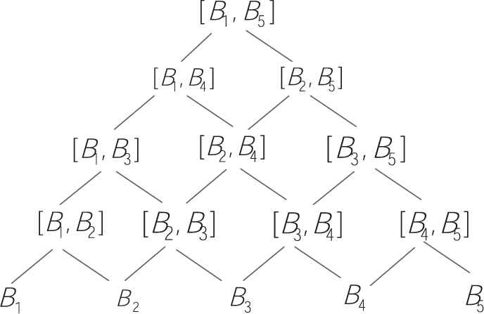
According to the graph
The definition of distance between two linguistic expressions is also given (Definition 7).
Definition 7.
[31] The distance between two linguistic expressions
The function ψ maps a linguistic expression [Bi, Bj] as a point in the plane.
3. A NOVEL DISTANCE MEASURE BETWEEN HFLTSs
3.1. Characteristics of HFLTSs
The previously presented Hs in Definition 4 appears in as an interval form and it is viewed as an information granule. Information granules offer a unique way of quantifying a diversity of sources of knowledge under consideration and expressing this aspect in the form of the level of granularity (specificity) [32]. We apply two criteria parameters (coverage criterion and specificity criterion [32]) to describe the characteristics of Hs.
Definition 8.
[32] Characteristics of Hs are described by coverage index cov (Hs) and specificity criterion spe (Hs):
A coverage criterion cov (Hs) expresses to which extent Hs covers. It reflects the uncertainty degree of Hs.
A specificity criterion spe (Hs) articulates the cumulative length of Hs. It reflects the position of Hs in the domain S.
Let
The specificity index is expressed as
There are two decision scenarios. The first one is that decision makers use multi-granular linguistic term sets to discriminate the assessments with different precision levels. That is to say, decision makers are free to choose elements of different coverage criteria. The other one is that a decision maker chooses one linguistic term set and use several elements in this set to generate different HFLTSs to discriminate the assessments with different precision levels, just like HFLTSs in Definition 2. According to Definition 2, Hs is generated from
3.2. A Weighted HFLTSs Graph
The distance between two HFLTSs is defined as the geodesic distance in the graph
Definition 9.
Given a weighted graph
Let us consider the vertices set.
We group the vertices according to cov (xi,j). The same group is at the same “cover”. We use ∧t to describe a group that represents the same coverage index. ∧t will be:
The graph
Definition 10.
A graph
For example,
In the graph
Then, let us see the edges set
Finally, we look at the weight set
3.3. The Distance Measure Between HFLTSs
Note that each edge of a graph may have a specific weight
Roselló, Prats [34] used an information function of qualitative labels to measure the consensus degree of two qualitative labels in the group decision. We modify this function to measure the distance between two linguistic intervals. The information I for the vertex xi,j is a positive continuous real function. It is used to build the weight function of each edge. The information I satisfies that if xi,j and xh,k are two vertices and
Definition 11.
The weight function
Remarks.
k reflects the importance of imprecise when deciding the weight of an edge. If two vertices are more different in coverage, then
In our model, an edge is between two close neighbor levels. Since every vertex in a level is uniform distributed, we can get
Hence, the weight of the edge between level Λt and Λt+1 is
Corollary 1.
If k = 0, the distance of all edges in the space
The weight function (9) calculates the distance of two directly connected vertices. Now we introduce an approach to calculate the distance from arbitrary vertices v0 to vk. There are several possible reachable paths from vertex v0 to vk, and a path is denoted as a finite sequence p = v0v1 … vk, where vi ∼ vi+1 is an edge. The path length of the path p is denoted as
Corollary 2.
If the weights of all edges in the space
Proof.
The shortest path is the union of two parts. xa,j and xr,s are in the same level. xa,j is between xi,j and xr,s in vertical direction.
Without loss of generality, we assume r ≥ i and s ≥ j. See Figure 2.
An example to show the positions of vertices xi, j and xr, s.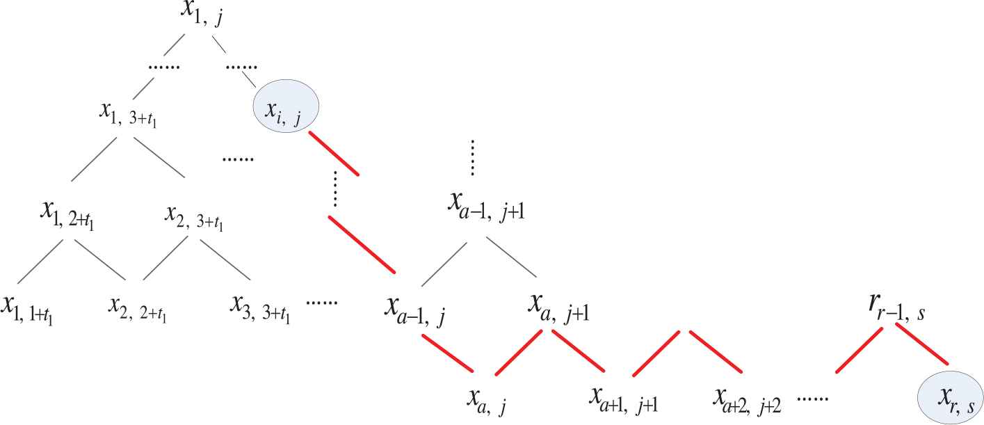
The red lines in Figure 2 are the shortest path from xi,j to xr,s. The path can be divided into two parts. One path is vertical and the other is horizontal. The vertical part is from xi,j to xa,j, and the horizontal part is from xa,j to xr,s. These two paths constitute the shortest path from xi,j to xr,s.
The shortest path from xi,j to xa,j is a straight line. The distance of this line is
The shortest path from xa,j to xr,s is like a zigzag line. The distance of this line is
The whole distance from xi,j to xr,s is
Other situations can be treated in a similar way. So we conclude:
Remarks.
We can conclude from Corollary 2 that in a special situation our distance measure coincides with Function (4). In other words, Function (4) is equal to our distance measure when k = 0. k = 0 means that we do not consider the coverage criterion of characteristics of Hs. If we consider the coverage criterion of HFLTSs, our distance measure shows its advantage. In fact, the coverage criterion of HFLTSs is just what many other distance measures will ignore. After a deeper analysis of the characteristics of HFLTSs, it is seen that the coverage criterion of HFLTSs reflects the hesitance of decision makers. The hesitance of decision makers reflects personality and knowledge background, which is important for FGDM. A distance measure without fully considering the characteristics of HFLTSs is not perfect.
3.4. Comparison Operators
The comparison of HFLTSs represented by linguistic intervals is carried out according to an ordinary lexicographic order [27]. Lexicographic order is more intuitive for people.
Given
The binary relation
This order seems natural: the closer the assessments are to the linguistic term sg, the better the alternative is. The better alternative also has the longest geometric distance from s0. Then we give the proof.
Lemma 1.
For all
Proof.
Lemma 2.
For all
Proof.
4. APPLICATION TO FUZZY GROUP DECISION MAKING
4.1. The Description of FGDM
FGDM, which uses linguistic expresses as assessments, becomes an important research subject because of the fuzziness of objective things and hesitance of human thinking. Assume a set of decision makers
Decision makers use comparative linguistic expressions to express their assessments. The key problem in our decision process is in the aggregation phase. We need to aggregate
In this section, we will introduce an approach based on distance measures to solve FGDM problems.
4.2 The Aggregation Approach Based on Distance Measure
The basic assumptions of the aggregation approach are as following:
The result of aggregating a set of linguistic intervals is also a linguistic interval.
The linguistic interval should reflect all information of the set of linguistic intervals as accurately as possible.
In the aggregation phase, we find a linguistic expression which has the minimal distances from all assessments
Now we give the Algorithm 1 to find a linguistic expression which has the minimal distances with
Algorithm 1:
Step 1. Construct
Step 2. Calculate distance for ui.
For a starting node ui ∈ V, use Dijkstra’s shortest path algorithm to calculate the distance d(ui ∼ v) for all v ∈ V.
Step 3. Find the substitution xi,j.
We present the model based on the weighted averaging operator to find a linguistic expression having the minimal distances with
In the model, yi,j = 1 means that vertex xi,j is selected as the best substitution. The condition is that we can only select one node.
We can extend this model to meet the needs of some operators. Now we give an extension for the hesitant fuzzy LOWA (HFLOWA) operator.
A common extension operator is given as follows.
Since our models reach the result that has the minimal distances with
Definition 12.
Proximity degree function is defined by
In function (10), we find the vx in
Our aggregation approach not only solves the problems of aggregating decision makers assessments, but also gets the result with good proximity degree. So we think it is especially suitable for FGDM.
4.3 The Process of FGDM with HFLTSs
Based on the proposed algorithm of finding a substitute expression of HFLTSs, the proposed FGDM approach is presented as follows:
Step 1. Transform comparative linguistic assessment aij into HFLTS.
Use the transformation function EGH [10] to convert comparative linguistic expressions into HFLTS. The HFLTS is presented as
Step 2. Construct a graph for decision makers.
For all decision makers, all assessments are the vertices in graph
Step 3. Aggregate assessments of decision makers.
Given
Repeat Steps 2 and 3 until
We obtain
Step 4. Exploitation phase.
Establish a rank ordering among
4.4 Discussion and Comparative Analyses
Now we highlight some advantages of our approach with respect to others. We focus on two aspects:
Accuracy of the distance measure
In our approach, the distance measure is based on the Manhattan distance. Although most distances or similar measures are based on the Hamming distance and Euclidean distance, we think these kinds of distance measures cannot reflect the diversity of the linguistic intervals. The linguistic intervals cover different numbers of granule in S. Distance function in definition 5 adds linguistic terms in
Complexity of the aggregation model
It is universally acknowledged that the aggregation result of a set of hesitant fuzzy information should have the minimums difference with the set of hesitant fuzzy information. Different aggregation models realize this aim from different aspects. Rodriguez, Martinez [9] defined two aggregation operators, min_upper and max_lower, which carry out the aggregation by using HFLTS. These aggregators do not require that the cardinality of
5. ILLUSTRATIVE EXAMPLES
We use two examples to illustrate the process of our aggregation approach.
Example 11.
Consider two alternatives
| x1 | x2 | wi | |
|---|---|---|---|
| e1 | l4 | l3 | 1/3 |
| e2 | [l3, l4] | [l3, l4] | 1/3 |
| e3 | [l2, l4] | [l3, l5] | 1/3 |
Decision makers assessments of example 1.
The graph
We assume that the global opinion
When k = 0, the weight of any edge is
Using Lingo software, we obtain
The global opinions of the two alternatives are the same.
Since
Then we calculate the group consensus degree
Since δ1 = δ2, the proximity degrees of the two aggregation results are the same.
Example 2.
Consider two alternatives
| x1 | x2 | wi | |
|---|---|---|---|
| e1 | l2 | l3 | 1/3 |
| e2 | [l3, l4] | [l4, l5] | 1/3 |
| e3 | [l2, l5] | [l1, l4] | 1/3 |
Decision makers assessments example 2.
When k = 1, the weight of any edge is
The edge connecting the basic
The edge connecting the level ∧1 and ∧2 is
The edge connecting the level ∧2 and ∧3 is
The edge connecting the level ∧3 and ∧4 is
Construct model to find the substitution
Since
Then we calculate the group consensus degree
Since δ1 < δ2, the proximity degree of
Remarks: We apply
Roselló, Sánchez [31] computed the distances from optimal labels F and solved group decision-making under multi-granular linguistic assessments. With their method, we obtain the following result of Example 2:
This result is the same with ours.
Liao et al. [8] extended the shorter HFLTS to obtain the same length and compute the distances to rank alternatives in multi-criteria decision making. With their method, the solution for the problem in Example 2 is presented below:
Firstly, one can extend these preferences into the same length and get matrix
The hesitant fuzzy linguistic positive ideal solution is
Finally, we get
This result is the same with ours.
Hence, consistent ranking results are reached between our approach and that of Roselló et al. and Liao et al. for the problem in Example 2. However, the advantages of our approach with respect to others are highlighted in Section 4.4.
6. CONCLUSION
This newly developed distance measure can complement the existing computational models and is particularly suitable for solving FGDM problems in a context-free grammar. HFLTSs have diversity not only in center points but also in the coverage (degree of uncertainty). The most difficult problem when dealing with HFLTSs is aggregation because the coverage indices of HFLTSs are different. A proper operator is the key. We propose a new approach to get the aggregation result. The idea is the result should have the minimal distances with the HFLTSs. This idea is reasonable and consistent with the definition of proximity measure in GDM. This distance measure applied into FGDM is very suitable. And our numerical examples illustrate the process and effects of our method.
However, our distance measure assumes edges connecting the same two levels are of equal length. In fact, this condition is based on the assumption that the basic linguistic term set
CONFLICT OF INTEREST
This section is to certify that we have no potential conflict of interest.
This article does not contain any studies with human participants or animals performed by any of the authors.
ACKNOWLEDGEMENTS
This work was supported by National Natural Science Foundation of China (NSFC) (71871121, 71401078, 71503134), Top-notch Academic Programs Project of Jiangsu High Education Institutions, and HRSA, US Department of Health & Human Services (No.H49MC0068).
REFERENCES
Cite this article
TY  - JOUR
AU  - Mei Cai
AU  - Yiming Wang
AU  - Zaiwu Gong
AU  - Guo Wei
PY  - 2019
DA  - 2019/01/14
TI  - A Novel Comparative Linguistic Distance Measure Based on Hesitant Fuzzy Linguistic Term Sets and Its Application in Group Decision-Making
JO  - International Journal of Computational Intelligence Systems
SP  - 227
EP  - 237
VL  - 12
IS  - 1
SN  - 1875-6883
UR  - https://doi.org/10.2991/ijcis.2018.125905643
DO  - 10.2991/ijcis.2018.125905643
ID  - Cai2019
ER  -