
A New Edge Detection Method Based on Global Evaluation Using Supervised Classification Algorithms
- DOI
- 10.2991/ijcis.2019.125905653How to use a DOI?
- Keywords
- Image processing; Edge detection; Global evaluation; Edge segments; Supervised classification
- Abstract
Traditionally, the last step of edge detection algorithms, which is called scaling-evaluation, produces the final output classifying each pixel as edge or nonedge. This last step is usually done based on local evaluation methods. The local evaluation makes this classification based on measures obtained for every pixel. By contrast, in this work, we propose a global evaluation approach based on the idea of edge list to produce a solution that suits more with the human perception. In particular, we propose a new evaluation method that can be combined with any classical edge detection algorithm in an easy way to produce a novel edge detection algorithm. The new global evaluation method is divided in four steps: in first place we build the edge lists, that we have called edge segments. In second place we extract the characteristics associated to each segment: length, intensity, location, and so on. In the third step we learn the characteristics that make a segment good enough to become an edge. At the fourth step, we apply the classification task. In this work we have built the ground truth of edge list necessary for the supervised classification. Finally, we test the effectiveness of this algorithm against other classical algorithms based on local evaluation approach.
- Copyright
- © 2019 The Authors. Published by Atlantis Press SARL.
- Open Access
- This is an open access article distributed under the CC BY-NC 4.0 license (http://creativecommons.org/licenses/by-nc/4.0/).
1. INTRODUCTION
The edge detection technique is deserving an increasing attention in image processing. There is a huge class of algorithms that deal with this technique, but key formal/mathematical definitions are still needed. [1] The main goal of these edge detection algorithms is to identify those pixels with significant changes in their intensity—or more generally in their spectral information—respect to its pixels neighborhood.
In order to find these significant changes in an image, there are some algorithms that build their solution only by means of the information provided by adjacent pixels. [2, 3] Some other algorithms focus on the intensity changes of each pixel in a gradual way—or fuzzy—depending on the strength of the brightness gradient, for example. Once these intensity changes have been calculated, they classify the pixels as edge or as a nonedge, by means of some classical thresholding process made pixel by pixel. This strategy of decision is usually addressed as local evaluation [3, 4].
Due to the limitations of this local evaluation, in Ref. [5] was introduced the strategy of global edge evaluation. In that paper it was introduced the idea of edge list to break the independent decision made pixel by pixel. In this paper, we will refer to this edge list as a segment and it represents a collection of edge pixels connected in the image (see section 3). Nevertheless, similarly to the edge pixels, not all segments are good in the sense of segments that detect important luminosity changes in the image, being the bad ones those that mainly represent noise.
Based on this idea, in Ref. [6] it was presented a nonsupervised approach based on a fuzzy clustering technique to classify segments and decide the final edge detection solution. In order to deal with the segments classification problem in a supervised way, in Ref. [7] we developed a preliminary work to classify segments. In this paper, which is a more advance and complete version of Ref. [7], we try to learn what are the good segments by means of machine learning (ML) techniques. Nevertheless, any learning process needs a ground truth of the objects that have to be classified—in this case they are segments. It is important to emphasize that ground truth images are done pixel by pixel so it is necessary to build a new ground truth of segments. In order to do that, first the segments are built following a similar methodology to the one proposed in Ref. [5]. Once the segments are built, it is important to note that we do not know if they are good or bad for an edge detector task since all the ground truth are specifically designed for pixels and not for segments. Taking into account this, we decided to build the ground truth of the segments. This was made by means of computing the true positive (TP) pixels of each segment when matching against humans ground truth. The next step was to extract the relevant characteristics associated with each segment as the length, intensity average, dispersion, and position among many others (see Section 4, Step 2). In the final step we applied different supervised classification algorithms that allowed the discrimination between bad and good segments. Finally, and in order to test the effectiveness of the algorithm here proposed, we tested the edge segment detection-based algorithm with other classical edge detection algorithms using standard performance measures.
The remaining of this paper is organized as follows: The next section is dedicated to some preliminaries in edge detection problems and the evaluation techniques that will be used for the ground truth construction. The concept of global evaluation based on the concept of edge segment is presented in Section 3. In Section 4 the methodology for identifying relevant segments is proposed. Finally, in the last two sections, we present some results and conclusions, respectively.
2. PRELIMINARIES
In this section we remind some concepts related to edge detection and supervised classification.
2.1. Edge Detection Problems
From a mathematical point of view a digital image I can be viewed as the set of pixels defined below.
If
If
If
As it has been already pointed out, the main goal of edge detection algorithms is to detect those pixels in which the intensity change is significant.
From this idea it is clear that an edge detection algorithm transforms an image into a binary image. In this binary image, the white pixels (or one values) represent those pixels that have been identify by the edge detection algorithm as edge pixels. From a mathematical point of view the output of an edge detection algorithm is a function that converts a digital image into a binary image. We would like to emphasize that most of edge detection algorithms only deal with grayscale images although there are a high number of algorithms dealing with color images [8–10].
2.2. Edge Detection Steps
Many edge detection algorithms, follow some steps in order to build the possible edges of the image. We will use some of these steps to identify the candidate pixels to be edge, and from these candidates we will be ready to introduce the concept of segment. Any classical edge detection algorithm can be summarized with the following tasks:
Conditioning-preprocessing: During this first task the grayscale version—in our case we will be dealing only with grayscale images—of the original image I is well prepared for the next phases of edge detection. Traditionally it consists on smoothing, denoising, or some other similar procedure [11, 12]. In practice, this phase makes the edges easier to detect. After this phase, the result is a conditioned image that will be denoted as Is.
Feature extraction: The main aim of this step [13] is to build for each pixel
Taking into account previous consideration, for a given pixel
Blending-aggregation and thinning: During this phase, aggregating the information of the different features—directions—extracted into a single value denoted as edginess is most common. From now on, let us denote by
Scaling-evaluation: In this last step, it is necessary to obtain the final output that will be the binary image Ibin. Traditionally, each pixel has to be declared as an edge or as a nonedge pixel based on previous information. There exist many ways to discriminate between edge or not edge in this step. Some of them are based on thresholding accuracy assessment process [15]. Other authors [4] defined the concept of continuity and thinness based on a local edge evaluation method to decide between them. Other approaches based on Fuzzy Sets [16, 17] are possible.
Differences between local evaluation and global evaluation.
2.3. Performance in Edge Detection Problems
How to evaluate an edge detection algorithm is not a trivial task and there exist many approaches [18, 19]. In this work, we are going to follow the boundary-based evaluation methodology developed in Ref. [20, 21]. The methodology for benchmarking boundary detection algorithms developed by Ref. [21] is used on the Berkeley Segmentation Dataset (BSDS500). Nevertheless, this dataset of images was not created specifically for edge detection, but it is been used for edge detection comparisons these recent years [22]. This dataset consists of 500 natural images that are divided into a training set of 200 images, a test set of 200 images and a validation set of 100 images. Each image of BSDS is accompanied by a set of four to seven human-made reference boundary maps (see the “Humans ground-truth” in Figure 2) that serve as ground truth for evaluating the automatic boundary maps that constitute the output of an edge detection technique [20]. Given an image I and in order to compare an edge detection solution Ibin (a binary image) for this image with the result given by one human ground truth, a matching algorithm is developed to build the TP values and therefore the confusion matrix. In this matching algorithm a distance threshold δ is defined to specify the tolerance level to small boundary localization errors. Then, an unmatched automatic boundary pixel that lies closer than a distance δ from a human boundary pixel is counted as a TP). Otherwise, unmatched automatic boundary pixels are counted as false positives (FP). And unmatched human boundary pixels are counted as false negatives (FN). Once these values are obtained, the confusion matrix can be built as well as other accuracy measures as the precision (Prec), recall (Rec), and also the F-measure. These constitute the most accepted alternative in recent years (see Ref. [20, 22, 23]) to evaluate the performance of each one-to-one comparison.
From an original test image to the supervised algorithms output.
Formally, given a candidate automatic boundary map Ibin and a ground-truth human boundary map Igt, its comparison’s F-measure is computed as follows:
2.4. Supervised Classification Problems
The goal of supervised learning is to build a concise model to classify items into known classes in terms of predictor features. The resulting classifier is then used to assign class labels to the testing instances, where the values of the predictor features are known but the value of the class label is unknown. [24] It is possible to find a huge number of classification algorithms that have the common aim of maximizing the considered accuracy measures depending on a specific problem or dataset. In this paper we have focused on four well-known rule based classifiers such as classification and regression trees (CART) [24], random forest (RF) [25], stochastic gradient boosting (GBM), [26] and a more recent version of it called extreme gradient boosting (XGBoost) [27]. This last algorithm is widely used by data scientists to achieve the state-of-art results on many ML challenges. The main reason for this selection of algorithms is their capability of interpreting the results in terms of the predictor features. Since these four algorithms are based on rules, it is possible to understand the model created and even obtain a variable importance ranking.
3. GLOBAL EVALUATION: THE “EDGE SEGMENT” CONCEPT
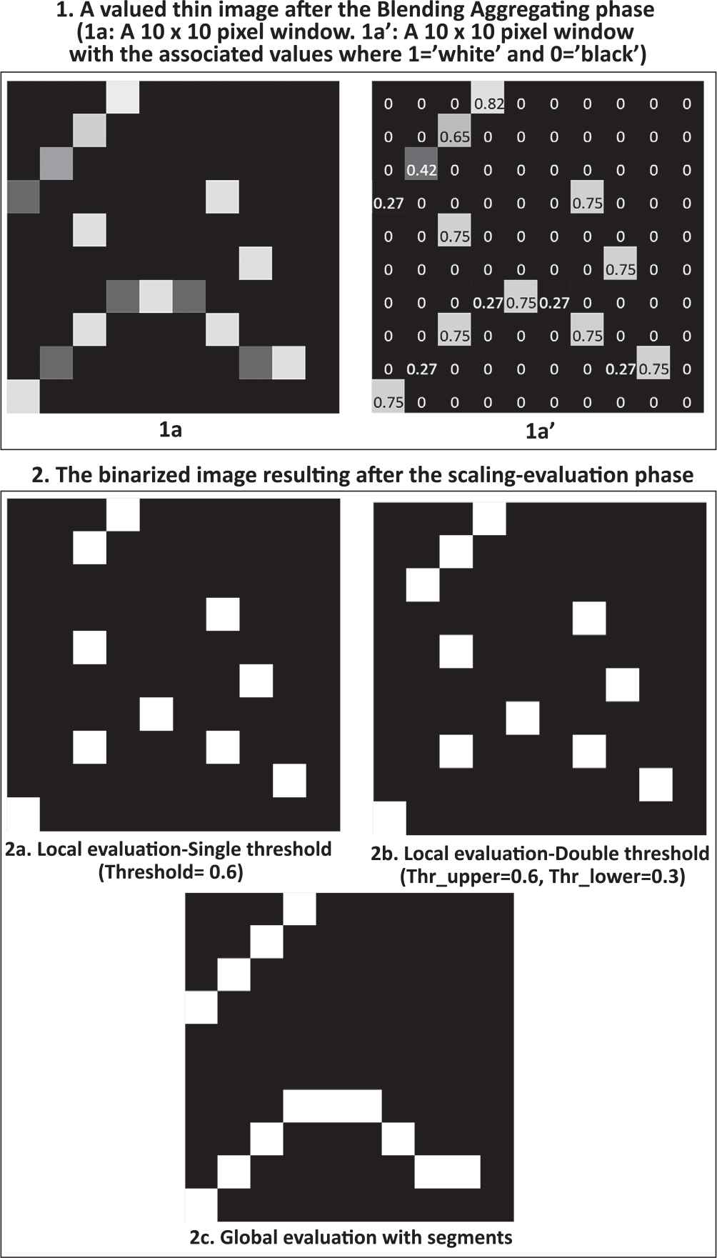
After the first three steps (see the “Previous phases of our work” points 0 through 3 at the top side of Figure 3), we will have a set of pixels that have been identify as possible edges (see and example in Figure 1.1). In this work, we will denote this set of pixels that are in fact candidates to be edges as
Flow diagram of our work.
Once the idea of the candidates to be edge C is defined, we can introduce the concept of edge segment. To explain with more detail what an edge segment is and to show its importance, let us remind that some authors [4, 5] have pointed out that something seems to go wrong when we decide to classify the candidates to be non-edge based on a local evaluation approach (see Figure 1.2a and b). Then, we propose the use of a global evaluation method over the pixels. More precisely, this approach is based on an evaluation over a list of connected pixels -linked edges- that will be refered later as edge segments. This idea of connection between pixels that are candidates to be edge lead us towards a fuller definition of this important concept that will be defined in the next paragraph:
Definition 1.
Let
S is connected, that is,
S is maximal, that is, if
Notice that, given this definition, each
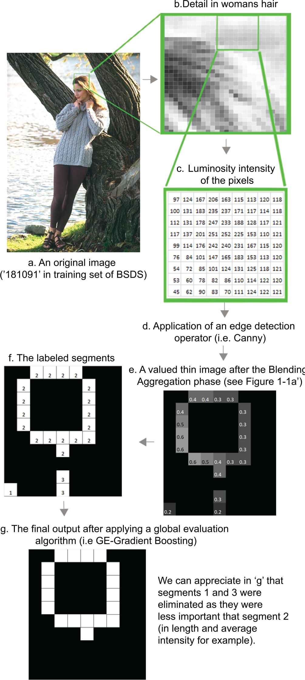
Another important consideration about the edge segments is that any candidate to become a final edge will not be just a single pixel, but the whole segment containing that pixel. This is the reason why in Figure 1.2 two whole segments are retained and in Figure 4 only one segment is retained. Now it is necessary to classify in a supervised way if one segment is good or not in order to learn what are the characteristics that permit this discrimination.
From the original image to the segments.
4. CLASSIFYING SEGMENTS IN A SUPERVISED WAY FROM AN EVALUATION FRAMEWORK
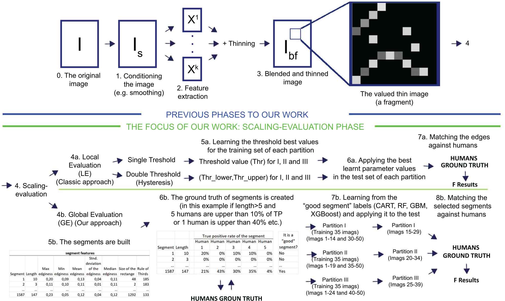
As we have said in the introduction, the main aim of this work is to provide a novel edge detection algorithm based on a global evaluation method. Our approach can be viewed as a global evaluation algorithm that can be applied after the three first steps of any classical edge detection algorithm. Taking into account this, in this section we will focus on the scaling-evaluation step of the algorithm (see the top half in Figure 3).
Once the segments have been identified in the image as we have explained in Section 3 (see Figure 4), it is necessary to classify them into two classes in order to complete the last phase of our edge detection algorithm. Many segments produced in this step can be considered as bad ones in the sense that they correspond to noise or non-relevant pixels. With this classification scheme, we want to know if it is possible to discriminate rightly based on its characteristics (length, intensity, dispersion, location, etc.). In Ref. [5], this discrimination process is done by clustering -which is an unsupervised approach- based only in two characteristics (length and average intensity). The main reason to present a supervised methodology is that we need to know if a segment is good or not in order to learn (based on its characteristics) how to discriminate between good and bad segments.
Hence, in this paper we propose to build a ground truth of segments based on the evaluation method proposed in Ref. [20, 21] Let us note that from this evaluation methodology, and based on the ground truth of edges, it is possible to have a measure for each segment by calculating the number of pixels that are true positive when comparing with humans ground truth. With this information we should be able to decide which segments are good and bad, as shown below. This whole process can be seen easily in the below part of the Figure 3.
Step 0. Choose an edge detection algorithm A.
Step 1. Building the segments. Given a dataset of images (in this work we have taken the Berkeley dataset [21]) we can build a set of segments after applying the first three steps of the algorithm A.
Step 2. Feature extraction from the segments. For each segment we obtained the following variables:
Length. For each segment Sl,
Therefore, it can be seen as the number of pixels in the segment.
Intensity Mean. For each segment Sl,
Where
Maximum and Minimum edginess. For each segment Sl, we obtained:
Standard deviation of the intensity. For each segment Sl:
“Rule of thirds” position. For each segment Sl, we obtained the coordinates of the pixel that occupies the central position in the segment:
Where
Once the gravity center is computed we get its euclidean distance to the intersection points following the rule of thirds, which is an standard in photography composition. [28] This rule establishes that the most important objects in an image are usually placed close to the intersection of the lines that divide the image in three equal parts. Following this principle, we computed the minimum of its four distances, as there are four intersection points created by these four lines.
Step 3. Building the ground truth dataset. The set of segments will be classified as good or bad according to the following procedure. For each segment it is possible to obtain the number of pixels that are matching as a true positive (TPl) for a specific human. Taking this information into account and looking forward to go beyond our last work [7], we decided to create different grades in which the segments had at least a certain percentage of positive matched pixels when comparing with a specific human. As the length of the segment could affect the importance of this percentages (e.g., in a four pixels length segment a 75% of true positive pixels could be non-relevant) this characteristic was used to compute the lower confidence interval (CIlow) of a Bernouilli distribution: Be(lengthl, %TPl). The different values of CIlow considered were seven—we called it “7levels”—10%, 15%, 20%, 25%, 30%, 35%, and 40%. Only in a few cases were considered five different levels—we called it “5 levels”—(from 20% through 40%) instead of seven. In all the cases, we considered as a perfect starting point or first level for this %TPl scale a 10%, as it kept a good balance between good and bad segments. When we went lower in the %TPl scale till reaching a 5% it did not work later in the comparatives. This is due specially to the almost perfect balance between good and bad segments which could limit the discrimination potential of the classifier. Therefore, depending of these CIlow values, the grade of matching of a certain segment could ranged from zero (CIlow < 10%) to seven (CIlow ≥ 40%). As there are five different humans, the human-aggregated level for a segment could range from 0 to 35. These aggregated level can be considered as an index that measures how true is a certain edge segment for the humans. Finally, in order to build the ground truth for all the segments analyzed we considered a segment Sl as “good” if the human-aggregation level of true positives was greater than a certain integer value. For example if this aggregation value is greater or equal to 5 we say that the supervised algorithm is an algorithm of “Aggregation 5.” The higher the aggregation value the more difficult for the segment to be good as it needs a high rate grade by the humans to be considered as a true edge segment.
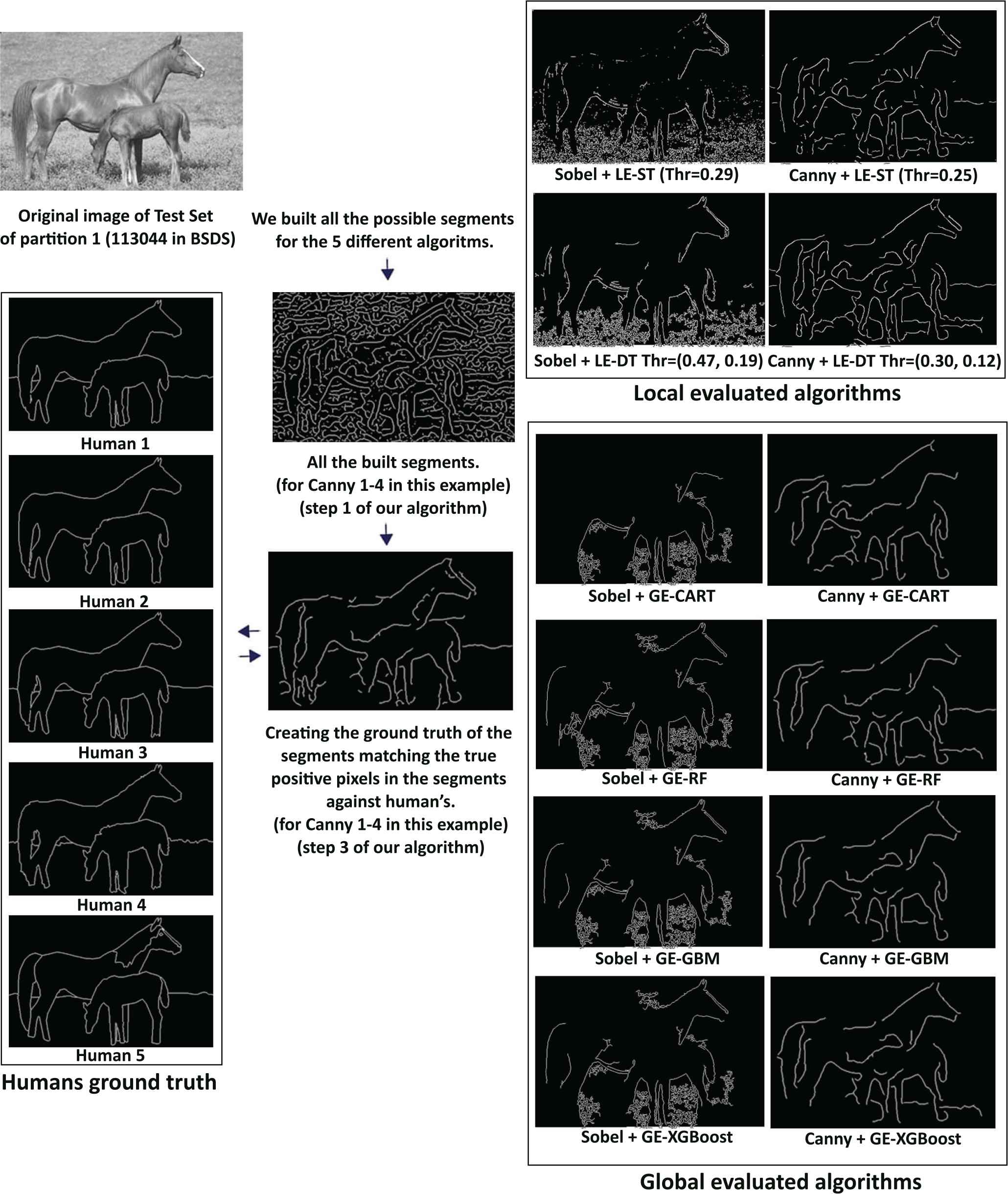
We can see a visual example of the creation of the ground truth of segments in Figure 3.6b. As well, we can see all the selected segments in the final ground truth in Figure 2. After this step, each segment was labeled as good or bad and we used this information in the supervised classification step (Step 5). Then, we created different versions of the ground truth for each algorithm -as the characteristics of the selected segments for each algorithm were slightly different. As well, we tried with different combinations of Lengthl and human-aggregated levels (from 5 to 15) and then we decided that Lengthl > 5 showed interesting results for all the algorithms. We found as well that the best human aggregation level ranged from 1 to 5 depending of the algorithm.
Step 4. Partition set of images. At this point we apply a dataset partition approach based on images. The segments of the training images will be classified (taking into account the human information) as good or bad (as we have said in the Step 3) and we will use this information to classify (by mean of a ML algorithm) the rest of the segments of the test images.
Firstly, we built the training set with 35 images and the test set with the remaining 15.
In order to avoid the possible over-learning from this partition, we repeated this process three times. Therefore, the results are shown by means of the three train/test partitions.
Step 5. Classification task-Learning. Given a ML algorithm and the segments that belong to the training images that has been classified into bad or good, it is possible to build rules based on the characteristics of Step 2 that permits to classify new segments (that belong to the test images) into bad or good.
Step 6. Classification task-Validation. With the classifier obtained in the previous step, all the segments of the test set are classified and classical accuracy measures are obtained. Specifically, we employed the area under ROC curve (AUC) as the metric to be improved in the training step because of the imbalance character of the created dataset. We can see this at Table 1.
| Canny 0-2 Ag 5-7levels | Canny 1-2 Ag 5-7levels | Canny 0-4 Ag 5-7levels | Canny 1-4 Ag 5-7 levels | Sobel 1 Ag 1-8 levels | |
|---|---|---|---|---|---|
| Good segments | 13.6 | 14.3 | 18.9 | 21.1 | 19.8 |
| Bad segments | 86.4 | 85.7 | 81.1 | 78.9 | 80.2 |
Segments balance for the algorithms (%).
5. COMPARATIVES AND RESULTS
In order to prove that our global evaluation approach gives better results than local evaluation, we chose 5 different edge detection algorithms in the first three steps. We have called these five algorithms as: Canny 0-2, Canny 1-2, Canny 0-4, Canny 1-4 and Sobel 1 based on the parameters values of Gaussian smoothing (σsmooth) and 'sigma of Canny’ (σCanny), which is the Gaussian filter that works in the convolution of Canny’s. [2]
Canny 1-2. Canny with σsmooth = 1 and σCanny = 2.
Canny 0-2. Canny without smoothing (σsmooth = 0) and σCanny = 2.
Canny 1-4. Canny with σsmooth = 1 and σCanny = 4.
Canny 0-4. Canny without smoothing (σsmooth = 0) and σCanny = 4.
Sobel 1. Sobel with σsmooth = 1.
For each one of these five algorithms we have used six different evaluation methods: two local evaluation methods (single and double thresholding) and four global evaluation methods based on four different ML algorithms (CART, RF, GBM, and XGBoost) that work with segments instead of pixels.
We have taken the first 50 images—sorted by number from 100075 to 16052—of the Berkeley training set [21]. For all the images, we built the set of candidates C and their associated segments sets as done in Ref. [5]. From these 50 images we have obtained a different amount of segments depending of the algorithm applied and its characteristics
A total of 115.580 segments for Sobel 1.
A total of 85.560 segments for Canny 1-2.
A total of 45.997 segments for Canny 1-4.
A total of 92.620 segments for Canny 0-2.
A total of 47.719 segments for Canny 0-4.
Not all of these 387.476 segments—the sum of the segments for the five different algorithms—were used in the learning process, but only the segments with length > 5 that finally were 40.752 (35%), 35.627 (42%), 19.508 (42%), 20.039 (42%), and 38.251 (41%), respectively. We can see a visual example of one of these buit ground truth (for Canny 1-4) in the middle of Figure 2.
Once the dataset was created, we split it into train/test partitions, and repeated this process three times. For each training set we fitted the four selected algorithms (CART, RF, GBM, and XGBoost), tuning the available parameters by means of a repeated cross validated learning process. Then, we were able to predict the test set and extract the ranking of the most important segment characteristics as it is showed in Table 2. We repeated the previous process three times in order to obtain a more robust values of accuracy measures and variables importance. We would like to emphasize that in this specific case the supervised classification task was not a trivial process for many reasons. Firstly, because we were dealing with a significant imbalanced classes dataset as we can see in Table 1, something that usually adds complexity to the training step. The second reason it was related to the overlapping between classes. In addition, the construction of the ground truth that could be difficult to fit and, moreover, having to do this for each algoritm.
| Canny 0-2 Ag 5-7 levels | Canny 1-2 Ag 5-7 levels | Canny 0-4 Ag 5-7 levels | Canny 1-4 Ag 5-7 levels | Sobel 1 Ag 1-8 levels | Total Average | |
|---|---|---|---|---|---|---|
| Maximum edginess | 1.75 | 2.00 | 1.25 | 1.00 | 1.00 | 1.40 |
| Mean edginess | 2.25 | 2.00 | 1.75 | 2.00 | 4.00 | 2.40 |
| Rectangle area | 3.00 | 3.25 | 5.25 | 5.50 | 4.00 | 4.20 |
| Rule of thirds distance | 4.00 | 4.00 | 4.50 | 4.50 | 4.25 | 4.25 |
| Standard deviation edginess | 6.50 | 6.50 | 4.25 | 3.50 | 2.50 | 4.65 |
| Minimum edginess | 5.75 | 5.50 | 4.75 | 5.50 | 5.75 | 5.35 |
| Length of the segment | 5.50 | 5.50 | 6.50 | 6.75 | 6.50 | 6.15 |
Values in bold refer the average ranking of five most important variables
Variables importance ranking for the algorithms.
As we can see at the variables importance ranking in Table 2, maximum edginess, mean of edginess, the area of the rectangle containing the segment, the “Rule of thirds” points distance to the center (related with the position of the segments in the image), and “Std. deviation of edginess” were the five most important characteristics.
We present in Table 3 the F results of the test set of partition 1 for the different algorithms studied. The rest of the tables (from Tables 4 through 8) are average of three partitions, being each partition results like the Table 3. In this sense, Table 3 is shown as an example for understanding how exactly the F measures of the rest of the tables are computed. In Figure 2, we can see a visual example of the algorithms output. As the dataset of images uses several human reference for each image—from 4 to 8—the F-maximum of the humans, their F-mean, and their F-minimum were considered separately as they provide different information and meanings. As can be seen in Tables 4 through 8 the five algorithms used in this work—each one with its results table—have been applied with six different algorithms versions. Two of them local evaluated: single threshold (ST) and double threshold (DT), and other four global evaluatedf versions (GE) with the four supervised algorithms employed (CART, RF, GBM, and XGBoost). The F-measure results for supervised algorithms with global evaluation along the new tables show a relevant improvement compared with previous work [7]. Local evaluated Canny and Sobel supervised algorithms were outperformed by our classification methodology based on global evaluation—segments—by the four algorithms employed. In more detail, we can appreciate that all these four supervised algorithms were closer to the humans in average, especially for Canny algorithms. Two of these algorithms (GBM and XGBoost) were the closest to any human (which is shown by the F maximum), and all of them were the closest to the more different human (which is shown by the F minimum) but for Sobel’s.
| Images (BSDS 500) | LE-ST (Thr =0.25) | LE-DT Thr =(0.28, 0.11) | GE-CART | GE-RF | GE-GBM | GE-XGBoost |
|---|---|---|---|---|---|---|
| 113016 | 0.64 | 0.61 | 0.72 | 0.67 | 0.69 | 0.68 |
| 113044 | 0.56 | 0.56 | 0.61 | 0.64 | 0.64 | 0.65 |
| 117054 | 0.55 | 0.51 | 0.54 | 0.57 | 0.60 | 0.60 |
| 118020 | 0.47 | 0.50 | 0.45 | 0.51 | 0.49 | 0.50 |
| 118035 | 0.62 | 0.62 | 0.59 | 0.57 | 0.63 | 0.66 |
| 12003 | 0.43 | 0.38 | 0.50 | 0.51 | 0.50 | 0.50 |
| 12074 | 0.40 | 0.39 | 0.43 | 0.41 | 0.43 | 0.43 |
| 122048 | 0.41 | 0.41 | 0.34 | 0.35 | 0.35 | 0.34 |
| 124084 | 0.47 | 0.49 | 0.46 | 0.46 | 0.47 | 0.47 |
| 126039 | 0.49 | 0.50 | 0.48 | 0.48 | 0.45 | 0.45 |
| 130034 | 0.25 | 0.25 | 0.38 | 0.32 | 0.35 | 0.36 |
| 134008 | 0.36 | 0.29 | 0.40 | 0.42 | 0.45 | 0.47 |
| 134052 | 0.52 | 0.48 | 0.55 | 0.54 | 0.54 | 0.54 |
| 135037 | 0.32 | 0.34 | 0.36 | 0.35 | 0.36 | 0.36 |
| 135069 | 0.85 | 0.82 | 0.88 | 0.88 | 0.88 | 0.88 |
| F Mean of the 15 images | 0.49 | 0.48 | 0.51 | 0.51 | 0.52 | 0.53 |
Values in bold refer the algorithm with the highest performance for that image
Humans F-mean for each image in partition I for Canny 1-4 (σsmooth = 1 and σCanny = 4).
| Algorithms | Humans Mean | Humans Min | Humans Max |
|---|---|---|---|
| Canny 0-2 + LE-ST (Thr=0.29 for I,III;Thr=0.30 for II) | 0.44 | 0.34 | 0.54 |
| Canny 0-2 + LE-DT(Thr=(0.39,0.16) for I,III; Thr=(0.42,0.17) for II) | 0.43 | 0.34 | 0.54 |
| Canny 0-2 + GE (Agreg=5, 7 levels)-CART | 0.45 | 0.36 | 0.55 |
| Canny 0-2 + GE (Agreg=5, 7 levels)-RF | 0.45 | 0.37 | 0.55 |
| Canny 0-2 + GE (Agreg=2, 7 levels)-GBM | 0.45 | 0.36 | 0.56 |
| Canny 0-2 + GE (Agreg=5, 7 levels)-XGBoost | 0.45 | 0.36 | 0.55 |
Values in bold refer algorithm with the highest performance for a specific human agregation
F average of the three test set partitions for Canny 0-2 (σsmooth = 0 and σCanny = 2).
| Algorithms | Humans Mean | Humans Min | Humans Max |
|---|---|---|---|
| Canny1-2 + LE-ST (Thr1=0.28 for I and III,Thr=0.29 for II) | 0.45 | 0.35 | 0.55 |
| Canny1-2 + LE-DT(Thr=(0.39,0.16) for I,II; Thr=(0.42,0.17) for III) | 0.45 | 0.35 | 0.55 |
| Canny1-2 + GE(Agreg=5, 5 levels)-CART | 0.46 | 0.38 | 0.57 |
| Canny1-2 + GE(Agreg=5, 5 levels)-RF | 0.47 | 0.38 | 0.60 |
| Canny1-2 + GE(Agreg=5, 7 levels)-GBM | 0.47 | 0.38 | 0.57 |
| Canny1-2 + GE(Agreg=5, 7 levels)-XGBoost | 0.46 | 0.38 | 0.57 |
Values in bold refer algorithm with the highest performance for a specific human agregation
F average of the three test set partitions for Canny 1-2 (σsmooth = 1 and σCanny = 2).
| Algorithms | Humans Mean | Humans Min | Humans Max |
|---|---|---|---|
| Canny0-4 + LE-ST (Thr=0.23 for the three partitions) | 0.46 | 0.36 | 0.57 |
| Canny0-4 + LE-DT(Thr=(0.29,0.12) for I; Thr=(0.31,0.12) for II,III) | 0.46 | 0.36 | 0.57 |
| Canny0-4 + GE(Agreg=5, 7 levels)-CART | 0.49 | 0.39 | 0.58 |
| Canny0-4 + GE(Agreg=5, 7 levels)-RF | 0.49 | 0.41 | 0.59 |
| Canny0-4 + GE(Agreg=5, 7 levels)-GBM | 0.50 | 0.41 | 0.59 |
| Canny0-4 + GE(Agreg=5, 7 levels)-XGBoost | 0.50 | 0.41 | 0.59 |
Values in bold refer algorithm with the highest performance for a specific human agregation
F average of the three test set partitions for Canny 0-4 (σsmooth = 0 and σCanny = 4).
| Algorithms | Humans Mean | Humans Min | Humans Max |
|---|---|---|---|
| Canny1-4 + LE-ST (Thr=0.25 for the three partitions) | 0.46 | 0.36 | 0.57 |
| Canny1-4 + LE-DT(Thr=(0.28,0.11) for I,II; Thr=(0.30,0.12) for III) | 0.45 | 0.36 | 0.56 |
| Canny1-4 + GE(Agreg=5, 7 levels)-CART | 0.48 | 0.38 | 0.57 |
| Canny1-4 + GE(Agreg=5, 7 levels)-RF | 0.48 | 0.39 | 0.57 |
| Canny1-4 + GE(Agreg=5, 7 levels)-GBM | 0.49 | 0.40 | 0.58 |
| Canny1-4 + GE(Agreg=5, 7 levels)-XGBoost | 0.49 | 0.40 | 0.58 |
Values in bold refer algorithm with the highest performance for a specific human agregation
F average of the three test set partitions for Canny 1-4 (σsmooth = 1 and σCanny = 4).
| Algorithms | Humans Mean | Humans Min | Humans Max |
|---|---|---|---|
| Sobel1 + LE-ST(Thr=0.28 for I,Thr=0.33 for II and III) | 0.39 | 0.32 | 0.49 |
| Sobel1 + LE-DT(Thr=(0.46,0.18),Thr=(0.49,0.20),Thr=(0.41,0.16)) | 0.38 | 0.30 | 0.48 |
| Sobel1 + GE(Agreg=1, 7 levels)-CART | 0.39 | 0.31 | 0.49 |
| Sobel1 + GE(Agreg=1, 7 levels)-RF | 0.39 | 0.31 | 0.52 |
| Sobel1 + GE(Agreg=1, 7 levels)-GBM | 0.37 | 0.29 | 0.49 |
| Sobel1 + GE(Agreg=1, 7 levels)-XGBoost | 0.39 | 0.31 | 0.51 |
Values in bold refer algorithm with the highest performance for a specific human agregation
F average of the three test set partitions for Sobel 1 (σsmooth = 1).
In order to show the effectiveness of our new methodology when applied on the results given by the classical Canny algorithm with σsmooth = 1 and σCanny = 4 for each image contained in the test set of partition 1 (see Table 3), we have checked whether the statistical analysis supports our intuitions.This statistical checking has been widely used and also recommended for supervised classification comparatives as can be seen in Ref. [29–31].
Specifically, we employed the Wilcoxon rank test [32] as a nonparametric statistical procedure for making pairwise comparisons between two algorithms. For multiple comparisons, we used the Friedman-aligned ranks test to detect statistical differences among a group of results. Finally, the Holm post-hoc test [33] has been used to find the algorithms that reject the equality hypothesis with respect to the best approach (the one with lower ranking) as control method.
Table 9 clearly reflects the superiority of, at least, the best of our global evaluation approaches with respect to the local ones. In fact, the traditional local evaluation obtained the highest ranking values for both considered thresholds and the Holm post-hoc test confirms the statistical improvement of our method when comparing the best approach (XGBoost) against them.
| Algorithm | Ranking |
|---|---|
| Single threshold | 4.40 |
| Double threshold | 4.47 |
| GE-CART | 3.47 |
| GE-RF | 3.33 |
| GE-GBM | 2.70 |
| GE-XGBoost | 2.63 |
| p-val | 0.0186 |
| Holm single thr. | 0.0364 |
| Holm double thr. | 0.0388 |
Values in bold refer algorithm with the highest performance
Average rankings of the algorithms (aligned Friedman), associated p-values, and Holm test APV for each algorithm. Canny 1-4 (σsmooth = 1 and σCanny = 4).
Moreover, pairwise comparisons given by the Wilcoxon rank test, Table 10, shows the statistical improvement reached by almost all global evaluation methods with respect to the local evaluation algorithms.
| Comparison | R+ | R- | p-val |
|---|---|---|---|
| GE-CART vs. single thr. | 90 | 30 | 0.0832 |
| GE-CART vs. double thr. | 93 | 27 | 0.0571 |
| GE-RF vs. single thr. | 95 | 25 | 0.0438 |
| GE-RF vs. double thr. | 98 | 22 | 0.0288 |
| GE-GBM vs. single thr. | 102 | 18 | 0.0158 |
| GE-GBM vs. double thr. | 101 | 19 | 0.0184 |
| GE-XGBoost vs. single thr. | 100 | 20 | 0.0214 |
| GE-XGBoost vs. double thr. | 101 | 19 | 0.0184 |
Values in bold refer significant improvement of the global evaluation version of the algorithm against the non global (local).
Wilcoxon test to compare the bipolar tuning approaches (R+) against the base classifier (R−).
For this reason, we can say that our new edge detection methodology based on global evaluation and supervised classification algorithms clearly outperforms the classical local evaluation approaches at least, considering the Canny σsmooth = 1 and σCanny = 4.
6. CONCLUSIONS
The principal contribution of this paper has been the use of supervised classification techniques to improve previous works [5, 6, 34] based on algorithms using global evaluation procedures that were based on nonsupervised clustering techniques. In addition with this, and with the aim to apply supervised classification techniques, we built a new kind of ground truth where the objects were segments instead of pixels.
From the analysis of the results we can conclude that in general the problem of classifying good and bad segments is not a trivial classification problem but when this methodology is applied to edge detection problems we see that global evaluation approach it is better when comparing with local evaluated algorithms.
We are aware of this improvement has been reached by means of a modified ground truth version—based on segments—created from the Berkeley segmentation data set. This fact points out the idea of building from the beginning a new data set of images based on segments which with a high probability could lead to even better comparative results. This could be an interesting idea for future research in this flexible methodology based on segments.
We think that the variables importance ranking (see Table 2) seemed surprising for three reasons. Firstly, because length variable was not as relevant as in Ref. [5] was suggested, but we are aware to the fact that the length > 5 requirement for the segments in order to belong to the ground truth and the area of the rectangle containing the segment both could affect to this variable importance. Secondly, because maximum edginess was considered the most important variable which can be as well considered as a novelty that was not considered in Ref. [5]. And finally, because the ranking showed that the position of the segment is an important factor to consider in the learning process. Following this idea, one possible research line for the future could try to include more features related to the position of the segment, and going even further introducing features related to the shape of the segment.
We suggest for future research the possible use of other well-known supervised algorithms as SVM, Näive Bayes, PCA, MEM, and many others. We have used for the supervised classification task the R software version 3.2 and specifically the caret package [35] which allows the user to create a very complete training process for huge algorithms with a simple interface and a large number of available options. Let us note that the variables ranking have been obtained by using the varImp function included in this package.
ACKNOWLEDGMENTS
This research has been partially supported by the Government of Spain, grant TIN2015-66471-P, and by the Government of the Community of Madrid, grant S2013/ICE-2845 (CASI-CAM-CM).
REFERENCES
Cite this article
TY  - JOUR
AU  - Pablo A. Flores-Vidal
AU  - Guillermo Villarino
AU  - Daniel Gómez
AU  - Javier Montero
PY  - 2019
DA  - 2019/01/28
TI  - A New Edge Detection Method Based on Global Evaluation Using Supervised Classification Algorithms
JO  - International Journal of Computational Intelligence Systems
SP  - 367
EP  - 378
VL  - 12
IS  - 1
SN  - 1875-6883
UR  - https://doi.org/10.2991/ijcis.2019.125905653
DO  - 10.2991/ijcis.2019.125905653
ID  - Flores-Vidal2019
ER  -