
Fusion of Measures for Image Segmentation Evaluation
- DOI
- 10.2991/ijcis.2019.125905654How to use a DOI?
- Keywords
- Image segmentation evaluation; Data fusion; Discrete Cosine Transform; Classifier model
- Abstract
Image segmentation is an important task in image processing. However, no universally accepted quality scheme exists for evaluating the performance of various segmentation algorithms or just different parameterizations of the same algorithm. In this paper, an extension of a fusion-based framework for evaluating image segmentation quality is proposed. This framework uses supervised image segmentation evaluation measures as features. These features are combined together and used to train and test a number of classifiers. Preliminary results for this framework, using seven evaluation measures, were reported with an accuracy rate of 80%. In this study, ten image segmentation evaluation measures are used, nine of which have already been proposed in literature. Moreover, one novel measure is proposed, based on the Discrete Cosine Transform (DCT), and is thus named the DCT metric. Before applying it in the fusion-based framework, the DCT metric is first compared with some state-of-the-art evaluation measures. Experimental results demonstrate that the DCT metric outperforms some existing measures. The extended fusion-based framework for image segmentation evaluation proposed in the study outperforms the original fusion-based framework, with an accuracy rate of 86% and a large Kappa value equal to 0.72. Hence, the novelty in this paper is in two aspects: firstly, the DCT metric and secondly, the extension of the fusion-based framework for evaluation of image segmentation quality.
- Copyright
- © 2019 The Authors. Published by Atlantis Press SARL.
- Open Access
- This is an open access article distributed under the CC BY-NC 4.0 license (http://creativecommons.org/licenses/by-nc/4.0/).
1. INTRODUCTION
Image segmentation is defined as the partition of an image into homogenous and meaningful constituent parts. These parts are referred to as segments. Image segmentation serves as a prerequisite step in object detection and computer vision systems. Hence, the quality of the image segmentation results has a direct impact on those systems. A lot of attention has been rendered to the development of image segmentation algorithms. However, evaluation of these algorithms has received far less attention. As a consequence, there is still no universally accepted measure for comparing the performance of various segmentation algorithms, or even different parameterizations of the same algorithm. In order to develop or improve segmentation algorithms, it is crucial to evaluate the quality of their results. In Zhang et al. [1], the importance of having application-independent methods for comparing results produced by different segmentation algorithms or different parameterizations of the same algorithm is stated in terms of: The need for autonomous selection from among possible segmentations yielded by the same segmentation algorithm, the need to place a new or existing segmentation algorithm on a solid experimental and scientific ground and the need to monitor segmentations results in real time.
Image segmentation evaluation is difficult due to the fact that image segmentation itself is a relatively ill-posed problem. Segmentation evaluation methods can be divided into subjective and objective methods. Subjective methods are based on the evaluation of segmentation results by human judges using intuition. This approach is time consuming and often leads to inconsistent results because humans have got varying visual capabilities of humans. Objective methods are divided into analytical, supervised and unsupervised methods [2]. Analytical methods do not evaluate the segmentation results. They directly evaluate the actual segmentation algorithms from a set of perspectives, e.g., the complexity, efficiency and execution time of a given algorithm. However, these properties usually do not have an impact on the segmentation results. Thus, analytical methods are not appropriate for evaluating the quality of segmentation results. Supervised and unsupervised methods analyze the segmentation results themselves. Supervised methods use a reference image called the ground truth to evaluate the segmentation results. They compare a given segmentation with the ground truth to assess the level of similarity between the two, and do not employ any prior knowledge. Unsupervised methods evaluate the segmentation results on the basis of some “goodness” parameters which are relevant to the visual properties extracted from the original image and the segmented image. Several objective segmentation evaluation methods have been proposed in literature [2]. However, they all have different functional underlying principals and thus make different assumptions about segmentations. As a result, they perform well in certain cases, and poorly in others. However, image segmentation evaluation problem can also be framed as a fusion problem. One way of doing this is by treating evaluation measures as independent sources of information or pieces of evidence, and then combining their outputs by means of a particular fusion strategy. The result obtained from using the combined measures is likely to be better than those obtained from using the measures as individuals. Application of information fusion in image segmentation evaluation has been reported recently. In the work of Zhang et al. [3] and Zhang et al. [4], a co-evaluation framework for improving segmentation evaluation by fusing different unsupervised evaluation methods was reported. Wattuya and Jiang [5] proposed an ensemble combination for solving the parameter selection problem in image segmentation. And a learning-based framework [6] was proposed that employs both supervised and unsupervised evaluation methods as features. Moreover, Peng and Veksler [7] proposed a method for selecting optimal parameters in interactive image segmentation algorithms based on the fusion of unsupervised evaluation measures. All these studies have demonstrated that data or information fusion improves performance.
Our contribution in this paper is two-fold. Firstly, a novel image segmentation evaluation measure based on the Discrete Cosine Transform (DCT) is proposed, which is called the DCT metric. Secondly, being an extended framework of Simfukwe et al. [8], this work employs ten image segmentation evaluation measures. The ten evaluation measures to be used in the extended fusion-based framework include the proposed DCT metric. These evaluation measures are served as features for training and testing five classifier models. The fusion-based framework evaluates a given segmentation as being either “good” or “bad”, as opposed to Zhang et al. [3, 4] and Lin et al. [6], where two segmentations are simply compared to each other to evaluate which one is better. Nevertheless, it is possible to have a scenario where the two given segmentations are both bad and therefore not suitable for use in the later stages of the application. In this study, the results reported by Simfukwe et al. [8] are used as the baseline. To the best of our knowledge, it is the only work in literature where a given segmentation is classified as being either “good” or “bad”.
The organization of this paper is as follows: some popular measures for the evaluation of image segmentation quality are presented in Section 2. The DCT metric and the fusion-based framework are described in Section 3. The experimental results are presented and discussed in Section 4. And in Section 5, conclusions and some possible future work are presented.
2. SUPERVISED IMAGE SEGMENTATION EVALUATION
A number of image segmentation evaluation methods have been proposed over the years. However, all of them are based on different functional underlying principles and make different assumptions about the image data/information. As a result, these measures perform well in some cases and poorly in others. Thus, each method has got its advantages and limitations [2]. It is therefore the duty of the system developers to choose the measure(s) that are suitable to their application. The following are some of the measures that are available in the literature.
H2 [9]: It is based on the fusion of Histogram of Oriented (HOG) and Harris features. Given a segmentation S and a ground truth G, the H2 compares the similarity/dissimilarity between their HOG and Harris features using Euclidean distance. A H2 score equal to 0 means that the segmentation is of perfect quality. H2 is based on Euclidean distance means that small perturbations in the HOG and Harris features’ values may result in a large Euclidean distance.
HOSUR [10]: It is based on the fusion of HOG and Speeded-Up Robust Features (SURF). Given a segmentation S and a ground truth G, the HOSUR compares similarity/dissimilarity between their HOG and SURF features using Euclidean distance. A HOSUR score equal to 0 means that the segmentation is of perfect quality. Since HOSUR is also based on Euclidean distance, small perturbations in the HOG and SURF features’ values may lead to a large Euclidean distance.
Boundary Displacement Error (BDE) [11]: It evaluates the quality of a segmentation by calculating the average displacement error of boundary pixels between a segmentation S and a ground truth G. This measure tends to penalize undersegmentation more heavily than oversegmentation, i.e. it exhibits bias towards segmentations with more segments [12].
Probability Rand Index (PRI) [13]: It takes a statistical perspective to segmentation evaluation. It counts the fraction of pairs of pixel labels that are consistent between the segmentation S and the ground truth G, taking the average across a set of ground truths so as to compensate for the scale variation of human perception. The PRI takes values in the range [0, 1]. A score value of 1 means that the segmentation is of perfect quality, whereas a score value equal to 0 means that the segmentation is of poorest quality. The disadvantage of the PRI is that it has a small dynamic range of [0, 1], thus its values across images and algorithms are often similar [14].
Variation of Information (VOI) [15]: It is based on information theory. This measure defines the discrepancy between a segmentation S and its ground truth G in terms of the information difference between them. A VOI score value equal to 0 means that the segmentation of perfect quality. Although VOI has some interesting theoretical properties, it tends to be unstable in terms of its perceptual meaning and applicability when multiple ground truths are used [16].
Global Consistency Error (GCE) [17]: It evaluates the degree of overlap between segments of a segmentation S and a respective ground truth G. Segmentations that are related in this fashion are deemed to be consistent because they could represent the image segmented at varying scales. A GCE value equal to 0 means that the segmentation of perfect quality. This measure does not penalize oversegmentation at all, but tends to heavily penalize undersegmentation [12].
Hausdorff Distance (HD) [18]: It evaluates segmentations by comparing the shapes of the segments in a given segmentation S and its respective ground truth G. A value of the object-level HD that is equal to 0 means that the segmentation is of perfect quality. The disadvantage of the HD is that it is only applicable to binary images, hence in an event that colored images are used, they must be converted to binary form [19].
Dice Index (DI) [20]: Given a segmentation S and its ground truth G, the DI is defined to compare the corresponding regions of S and G. The DI takes values in the range [0, 1]. A DI value equal to 1 means that the segmentation is of perfect quality, whereas a DI value equal to 0 means that the segmentation is of poorest quality. This measure is popular in biological and medical studies, and its efficacy in segmentation evaluation has not been extensively studied.
F1 Score (FS) [21]: It evaluates a segmentation S in terms of the degree of overlap between its objects and those of the respective ground truth G. An FS value equal to 1 means that the segmentation is of perfect quality. FS is most popularly used in machine learning, and its efficacy for evaluation of image segmentation quality has not been widely studied.
It can be seen that each measure has got its own disadvantages, and thus might perform well in some cases and poorly in others. In this paper, we decide to combine the measures so that they can compensate for each other’s weaknesses and compound each other’s strengths.
3. DCT METRIC
The DCT was first proposed by Ahmed et al. [22]. A 2-dimensional DCT can separate an image into different spectral sub-bands of varying importance, with respect to the image’s visual quality; i.e. most of the visually significant information about the image is concentrated in just a few coefficients of the DCT. For this reason, the DCT is widely used for image coding and is at the core of international standards such as the JPEG and MPEG.
The proposed DCT metric evaluates the quality of segmentation results by means of positive real-valued scores. It is based on the energy compaction property of the DCT; i.e. the ability of the DCT to store the bulk of the visually significant information of an image using only a few of its coefficients. The core of this metric is the assumption that a segmentation is expected to retain the visually significant information inherent in the original image, at all levels. Thus, our metric seeks to evaluate the discrepancy/similarity of the DCT coefficients of a segmentation and a given ground truth. Figure 1 depicts the structure of the DCT metric.
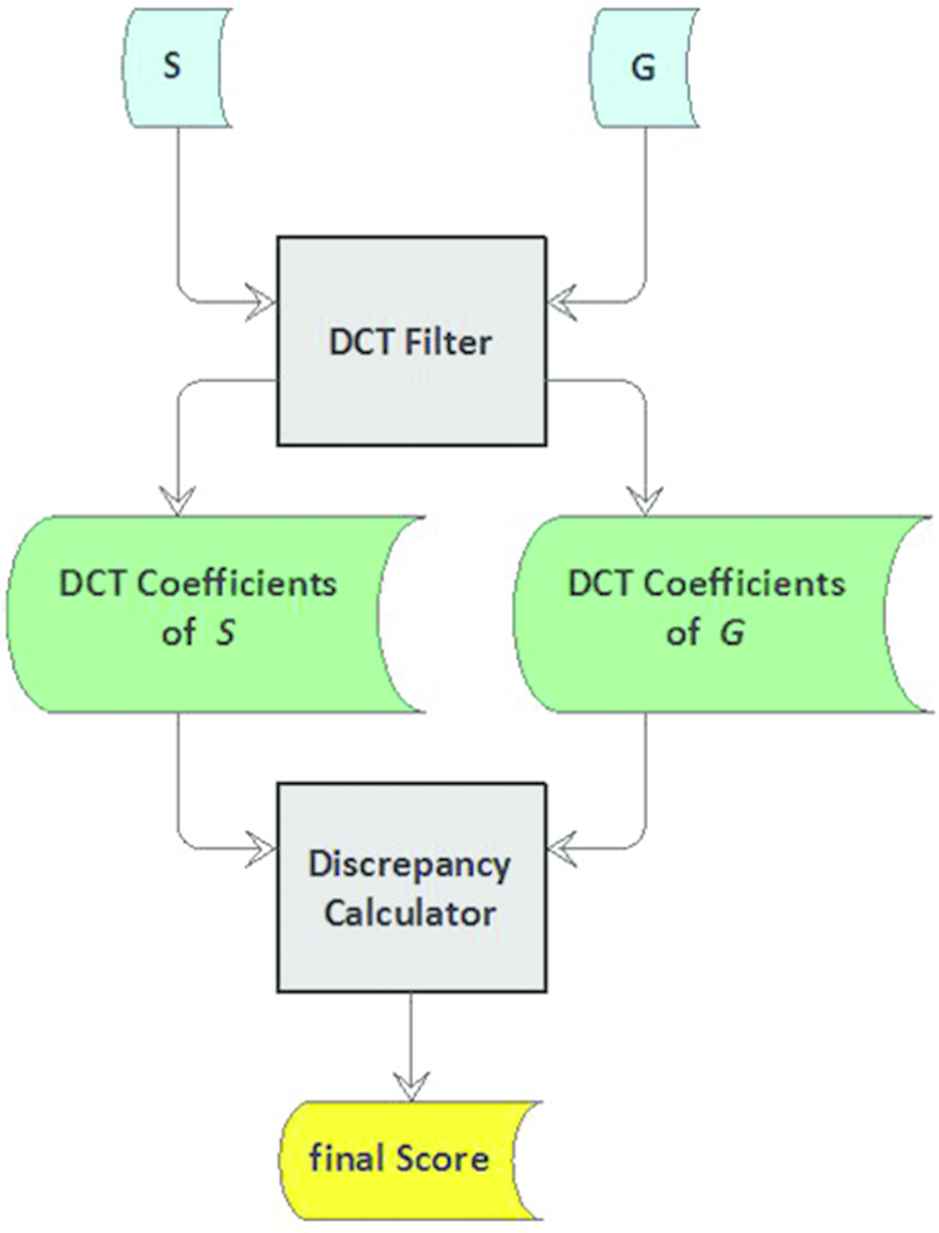
DCT metric’s schema
The DCT metric consists of two modules; the DCT filter and the discrepancy calculator. The DCT filter takes in a segmentation S and a ground truth G and produces DCT coefficients
The DCT metric produces a score value equal to 0 for a perfect segmentation. It has no upper bound.
4. FUSION-BASED FRAMEWORK
The proposed extended fusion-based image segmentation evaluation framework is presented in Fig. 2. It comprises two phases, namely the training and testing phases.
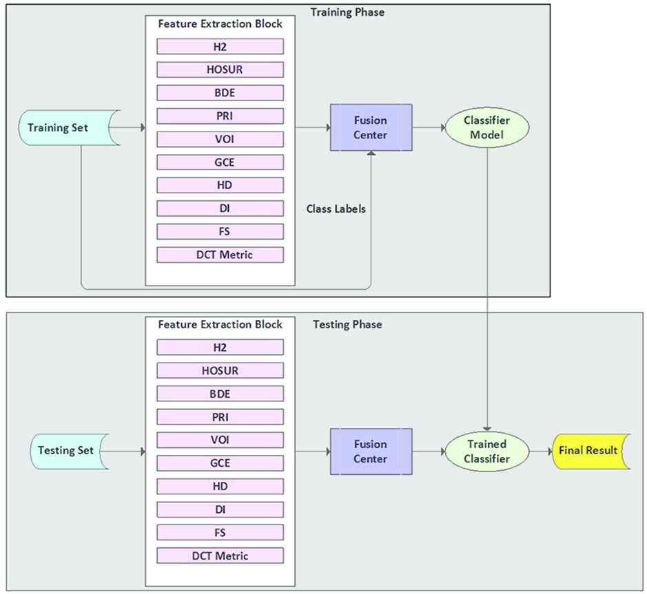
Extended fusion-based image segmentation evaluation framework
4.1. Training Phase
The training phase consists of four elements, namely the training dataset, the feature extraction block, the fusion center and the resultant trained classifier model. The training dataset contains the segmentations and their respective labels, assigned by human judges. Every segmentation is assigned a label of “good” or “bad”. The training dataset also contains the ground truths. For each segmentation, there are multiple ground truths that are representing the various perspectives of segmenting a given image, i.e. the differing opinions of the humans that produced these ground truths, on what a “perfect” segmentation should be. The segmentations are sent to the feature extraction block, which contains image segmentation evaluation measures of choice. For this study, ten image segmentation evaluation measures have been used; nine are from Section 2 and the tenth one is the DCT metric, proposed in Section 3. These evaluation measures are used as features that characterize the quality of segmentations on the basis of their score values.
The feature extraction block in Fig. 2 functions as follows. Given a segmentation S, a set of ground truths
The computed scores are sent to the fusion center. The fusion center combines the score values into feature vectors for the respective segmentations, e.g.
The training vector is obtained by combining the feature vector Z with the class label of a segmentation. The training vector is given as
4.2. Testing Phase
The testing phase comprises the test dataset, the feature extraction block, the fusion center and the trained classifier. The feature extraction block and the fusion center work in the same way as described in the training phase. The feature extraction block receives an unseen segmentation S, i.e. as segmentation that did not participate in training, from the test set. A set of ground truths
4.3. Classifier Models
In this study, we have used five classifier algorithms. Detailed descriptions about these algorithms can be found in Alpaydin [24] and Theodoridis and Koutroumbas [25].
Decision Tree (DT): The DT model is a classification model with the form of a tree structure. Each node is either a leaf node, which indicates the value of the target attribute (class) of examples, or a decision node. A decision node specifies some test to be carried out on a single attribute-value, with one branch and a sub-tree for each possible outcome of the test. Their advantage over other supervised learning methods lies in the fact that they represent rules, which are easy to interpret and understand and can also be readily used in a database.
Support Vector Machine (SVM): The SVM model is based on structural risk minimization. It finds a separator that maximizes the separation between classes and has demonstrated good performance in the various areas such as handwritten digit recognition, face detection, etc. SVM has excellent classification ability on small datasets and has high robustness. In our experiments, the SVM model with radial basis function serving as the kernel function was used.
Naïve Bayesian (NB): The NB model works on the assumption that the predictors, in our case the evaluation measures, are conditionally independent of each other. For our case two posterior probabilities are computed: the first one is the probability that a given segmentation S is good, given the attribute values, and the second one is the probability that S is bad, given the attribute values. Segmentation S is assigned to the class with the higher posterior probability. In our experiments, a NB model based on normal distribution was used.
K-Nearest Neighbor (KNN): The KNN model assigns the input to the class with most examples among the k neighbors of the input. All the neighbors have equal vote, and the class having the maximum number of voters among the k neighbors is chosen. In the case of ties, weighted voting is taken, and in order to minimize ties k is generally chosen to be an odd number. The neighbors are identified using a distance metric. In our experiments, the KNN model based on k = 4 and Correlation distance was used.
AdaBoost: AdaBoost belongs to a class of supervised learning approaches, collectively known as ensemble learning, which is basically about combining various learners to improve performance. In our experiments, 500 DTs were used as base learners, trained for 1 000 iterations.
5. EXPERIMENTAL RESULTS AND ANALYSIS
5.1. DCT Metric vs. Others
The proposed DCT metric is compared with other supervised segmentation quality evaluation measures, both subjectively and objectively. Subjective evaluation is carried out using the accuracy rate and objective evaluation is done with the help of Meta measures [26]. 200 images from the database presented in Lin et al. [27] are used for this task. Figure 3 shows some samples that are used, where the better segmentation in the pair as judged by humans is labeled in red.
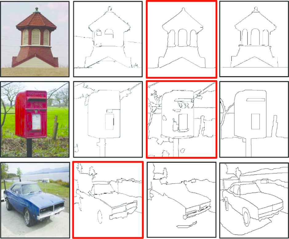
Sample images/segmentations from Lin et al. [27]. First column: Original image. Second column: Segmentation 1. Third column: Segmentation 2. Fourth column: Ground truth
The database contains two machine-generated segmentations for each image, labeled segmentation 1 and segmentation 2. It also contains multiple ground truths for each respective image. The aim is to let an evaluation measure decide which one of the two, between segmentation 1 and segmentation 2, is better than the other.
Table 1 shows the respective DCT metric scores for segmentations presented in Fig. 3. 1st Pair refers to the segmentations for the first image in the first column of Fig. 3, 2nd Pair refers to the segmentations for the second image in the first column of Fig. 3 and 3rd Pair refers to the third image in the first column of Fig. 3. The smaller the score value, the better the segmentation quality (The DCT metric yields a value equal to 0 for a perfect segmentation). From Table 1, it can be seen that the segmentations deemed to be of better quality by humans for each pair, have the smaller scores. This denotes the agreement between the decisions of the humans and the DCT metric, regarding the quality of the segmentations in Fig. 3.
| Segmentation 1 | Segmentation 2 | |
|---|---|---|
| 1st Pair | 1.20 | 0.21 |
| 2nd Pair | 3.80 | 1.02 |
| 3rd Pair | 1.46 | 2.56 |
DCT metric scores for segmentations from Fig. 3.
5.1.1. Subjective evaluation
A subjective comparison of the DCT metric with the BDE, VOI, GCE and PRI is conducted. For every image, there is a pair of segmentations and a ground truth, as shown in Fig. 3. For every pair of segmentations, 11 humans judge/determine which of the two segmentations is better. The segmentation that receives the majority votes is considered to be the better one. Further, the scores are computed for the segmentations in every pair using the DCT metric, BDE, VOI, GCE and PRI. Using these score values, it is then decided which segmentation in each pair is better. The accuracy rates for the measures are computed as
Table 2 shows the accuracy rate of the DCT metric in comparison to other measures. It can be seen that the proposed metric has a better performance than its counterparts.
| DCT metric | BDE | VOI | GCE | PRI | H2 | HOSUR | HD | DI |
|---|---|---|---|---|---|---|---|---|
| 96% | 85% | 92% | 90% | 95% | 95% | 92% | 89% | 90% |
Subjective comparison: DCT metric vs. other measures.
5.1.2. Objective evaluation
Meta-measures are used to evaluate the performance of the image segmentation evaluation measures. Pont-Tuset and Marques [26] proposed the following three meta-measures: Swapped-Image Human Discrimination (SIHD), State-of-the-Art-Baseline Discrimination (SABD) and Swapped-Image State-of-the-Art Discrimination (SISAD). A meta-measure must rely on an accepted hypothesis about the segmentation results and evaluate how coherent the evaluation measures are with such a hypothesis. An example of the hypothesis could be the human judgment of some segmentations and the meta-measure then serves as the quantization of how consistent the evaluation measures are with this judgment. This is the approach used in our experiments.
An objective comparison of the DCT metric with the BDE, VOI, GCE and PRI using the SIHD, SABD and SISAD. Table 3 shows the results of this comparison.
| DCT metric | BDE | VOI | GCE | PRI | H2 | HOSUR | HD | DI | |
|---|---|---|---|---|---|---|---|---|---|
| SIHD (%) | 96.1 | 85.4 | 94.9 | 94.6 | 95.8 | 95.4 | 92.2 | 89.3 | 91.1 |
| SABD (%) | 94.2 | 82.7 | 94.7 | 93.2 | 93.7 | 94.1 | 90.4 | 88.4 | 89.0 |
| SISD (%) | 91.7 | 78.2 | 80.2 | 89.1 | 90.6 | 92.3 | 89.6 | 88.0 | 89.0 |
Objective comparison: DCT metric vs. other measures.
From Tables 2 and 3, it can be seen that the DCT metric performs better than the other measures.
5.2. Fusion-Based Framework
The dataset utilized in our work is derived from the one used in Lin et al. [27]. It contains 1 000 different segmentations, with four to ten ground truths for every segmentation. The segmentations are machine-generated, while the ground truths are annotated by humans. In our derived dataset, all the segmentations are labeled “good” or “bad”. The detailed process of creating this derivative database is described in Simfukwe et al. [8]. Out of the 1 000 segmentations, 433 are labeled as “good” and 567 are labeled as “bad”. This means that the dataset is almost balanced (43.3% of the samples belong to one class and 56.7% belong to the other class). For the experiments, the dataset was divided into 700 training and 300 testing samples. Because our dataset is small, we adopted the experimental approach used by Chen et al. [28] and Zhang et al. [3], where the dataset was simply split into the training and testing (evaluation) sets, without a separate validation set. The other reason is that we wanted to maintain consistency with our baseline, as was stated in Simfukwe et al. [8], where the same dataset was also simply divided into 700 training and 300 testing samples, without a separate validation set. Further, we make sure that both the training and testing samples have the same distribution, i.e. 43% of the samples a labeled “good” and 57% of the samples are labeled “bad”.
The test set consists of both hard and easy cases, with respect to classification. Easy cases are those that were accurately classified by all the classifier models, while hard cases are those that were inaccurately classified by all or the majority of classifier models. Figure 4 shows the results for some easy and hard cases. For easy cases, the entire row of Table 4 contains either “Good” or “Bad”, depicting an agreement with the humans. The opposite is true for hard cases.
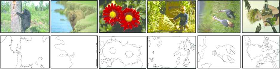
Easy and hard cases. First row: Original image. Second row: Segmentations
| Human | NB | DT | SVM | KNN | AdaBoost | Case | |
|---|---|---|---|---|---|---|---|
| 1st Column | Bad | Bad | Bad | Bad | Bad | Bad | Easy |
| 2nd Column | Bad | Bad | Bad | Bad | Bad | Bad | Easy |
| 3rd Column | Good | Good | Good | Good | Good | Good | Easy |
| 4th Column | Bad | Bad | Good | Bad | Good | Bad | Hard |
| 5th Column | Good | Bad | Bad | Bad | Good | Bad | Hard |
| 6th Column | Good | Bad | Bad | Good | Bad | Good | Hard |
Easy and hard cases.
During testing, the accuracy rate is computed by comparing the class label assigned to a given segmentation by the humans with the class label assigned to such a segmentation by the classifier. The accuracy rate is computed using Eq. (8) (where D is the number of times that the class label produced by the trained classifier is the same as that assigned by the humans, for a given segmentation. W is the total number of test samples, in this case W = 300).
The performance results for the proposed framework, in terms of accuracy rate, are presented in Table 5. It can be seen from Table 5 that the proposed framework has higher accuracy than when the measures are used individually to train the classifier models. This is confirmation that data fusion improves performance. The accuracy rate differences across the various classifier models for the same feature (image segmentation evaluation measure), is because of the fact that different classifier models are based on different functional principles and assumptions on the data. The best performance is produced by AdaBoost (86% accuracy rate), which is based on the concept of combining multiple classifier models. This serves as further confirmation that data fusion improves performance. There are no results from single features for DT and AdaBoost. This is because DT and AdaBoost models need more than one feature as input.
| H2 | HOSUR | BDE | PRI | VOI | GCE | FS | DI | HD | DCT metric | Proposed framework | |
|---|---|---|---|---|---|---|---|---|---|---|---|
| NB | 50% | 51% | 61% | 62% | 38% | 62% | 60% | 55% | 52% | 60% | 66% |
| SVM | 48% | 45% | 62% | 41% | 38% | 62% | 60% | 55% | 51% | 56% | 67% |
| KNN | 43% | 46% | 43% | 62% | 49% | 38% | 54% | 57% | 54% | 50% | 68% |
| DT | – | – | – | – | – | – | – | – | – | – | 64% |
| AdaBoost | – | – | – | – | – | – | – | – | – | – | 86% |
Accuracy rates: Proposed framework vs. individual measures.
It is also interesting to investigate the contribution of each evaluation measure towards the final accuracy rate of the framework. The baseline [8] employed the following seven measures: BDE, PRI, VOI, GCE, FS, DI and HD. In this study we investigated the marginal contribution of including the H2, HOSUR and DCT metric. It should be noted that the result presented in Table 5 are for the case when the H2, HOSUR and DCT are all included together with the measures from the baseline. Table 6 presents the accuracy rates when the H2, HOSUR or DCT metric are included in the framework together with the baseline measures. The baseline in Table 6 refers to the evaluation measures used in our baseline [8], i.e. the BDE, PRI, VOI, GCE, FS, DI and HD. It can be seen from Table 6 that the proposed framework outperforms the baseline for both cases, i.e. when the framework is extended by one evaluation measure and when it is extended by two measures. The inclusion of two evaluation measures produces better performance than the inclusion of one and the same is true when three measures are used, as shown by Table 5. This indicates that there is marginal performance improvement obtained from using more evaluation measures.
| Baseline | Baseline + HOSUR | Baseline + H2 | Baseline + DCT metric | Baseline + (HOSUR + H2) | Baseline + (HOSUR + DCT metric) | Baseline + (H2 + DCT metric) | |
|---|---|---|---|---|---|---|---|
| NB | 63% | 63.5% | 63.8% | 63.4% | 65% | 65% | 64% |
| SVM | 65% | 65.8% | 65.8% | 65.5% | 66% | 66% | 66% |
| KNN | 65% | 65.6% | 65.8% | 65.4% | 67% | 67% | 66% |
| DT | 61% | 61.9% | 61.9% | 61.6% | 63% | 63% | 62% |
| AdaBoost | 80% | 82.3% | 82.5% | 81.8% | 84% | 84% | 83% |
Accuracy rates: Baseline8 vs. proposed extended framework.
Sometimes it is not enough to make conclusions about the performance of a classifier only on the basis of accuracy. Several other methods have been proposed for evaluating classifier performance. One such method is the Kappa Statistic [29]. The Kappa Statistic measures the degree of agreement between the predicted and actual classifications, taking into account that there is a possibility that this agreement could be due to mere chance. The accuracy rate values presented in Table 5 are computed with respect to the labels assigned to segmentations by humans, and they reflect the frequency of agreement between the humans and the classifiers. However, it is important to determine whether this agreement is by mere chance or not, as well as the degree of significance of this agreement. The Kappa Statistic is employed for this task.
The Kappa Statistic is normalized and takes values in the range [0, 1]. A value equal to 1 means that there is perfect agreement, while a value equal to 0 means that the agreement is due to mere chance.
Observed accuracy refers to the frequency of correct predictions by a given classifier and it is equivalent to the accuracy rate defined by Eq. (8). Expected accuracy is the accuracy that any random classifier would be expected to achieve. For details on how to compute expected accuracy, please refer to Witten et al. [29]. Table 7 presents the Kappa values for the classifiers used in this study.
| Classifier | Kappa | Interpretation |
|---|---|---|
| NB | 0.34 | Fair agreement |
| SVM | 0.35 | Fair agreement |
| KNN | 0.34 | Fair agreement |
| DT | 0.31 | Fair agreement |
| AdaBoost | 0.72 | Substantial agreement |
Kappa values for classifiers.
It can be seen from Table 7 all the five classifiers agreement with humans is not as a result of mere chance (Kappa values are greater than 0 for all classifiers). NB, SVM, KNN and DT exhibit fair agreement with the humans. AdaBoost exhibits substantial agreement with the humans, further affirming the fact that it has the best performance among the chosen classifiers.
The results obtained in this study are compared to our baseline, which is the results presented in Simfukwe et al. [8]. It should be noted that the same framework was used in the baseline, but with fewer evaluation measures as features (only seven were used). In this study, ten evaluation measures have been used. However, the same classifier models were used in this study as in the baseline, i.e. NB, SVM, KNN, DT and AdaBoost. Figure 5 shows a comparison of results obtained in this study to those from the baseline [8], in terms of accuracy rate.
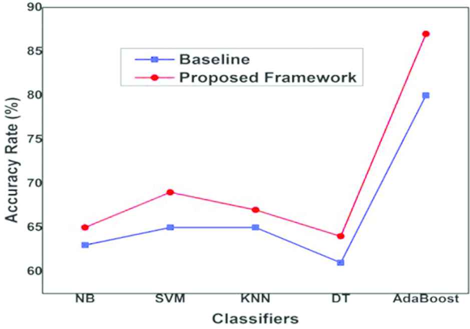
Accuracy rate: This study vs. baseline
The Kappa values can also be used to directly compare the performance of classifier models for a particular task. Figure 6 shows comparison of performance between the baseline and this study, in terms of the Kappa values.
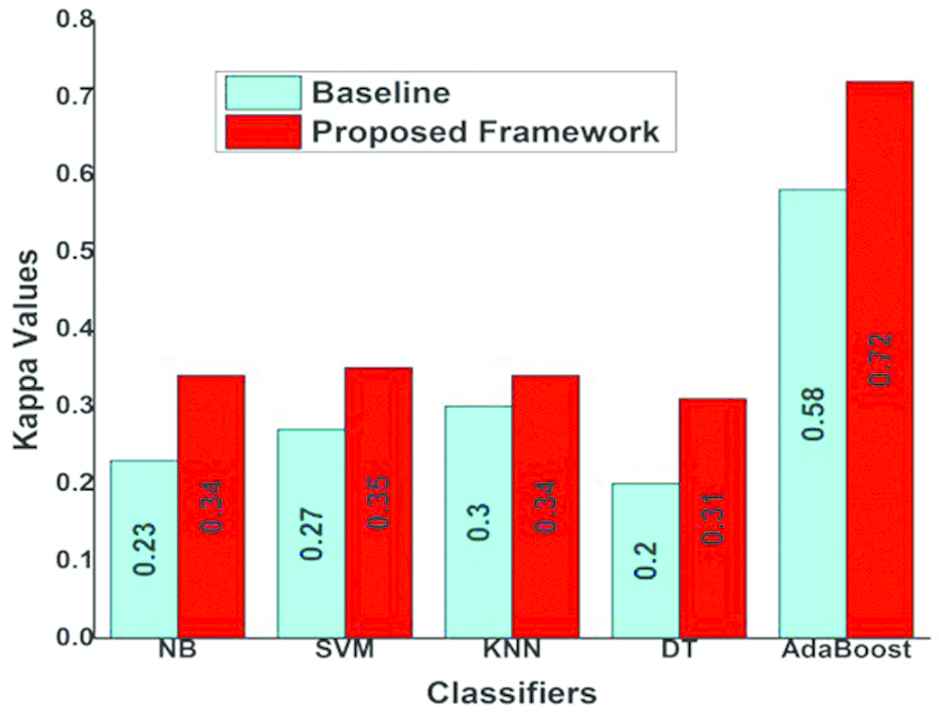
Kappa values: This study vs. baseline
From Figs. 5 and 6, it can be seen that there is improvement in the results obtained in this study in comparison to those obtained in the baseline, for all classifier models. This is because in this study ten evaluation measures, while the baseline used only seven. Therefore, it can be deduced that using more measures as features increases the likelihood of them supplementing each other, thus improving overall performance. This is the motivation behind data fusion.
6. CONCLUSION
In this paper, a novel measure for evaluation of image segmentation quality, called the DCT metric, has been proposed. This measure is based on the energy compaction properties of the DCT. The DCT metric employs a ground truth and thus belong to the category of supervised evaluation measures. Experimental results have shown that the DCT outperforms some popular image segmentation evaluation measures, i.e. BDE, PRI, VOI, GCE, DI, HD, HOSUR and H2.
An extended fusion-based framework for evaluation of image segmentation quality has also been proposed. This framework treats image segmentation evaluation as a binary classification problem, i.e. it classifies a segmentation as being either “Good” or “Bad”. The framework uses image segmentation evaluation measures as features to train five different classifier models. Experimental results for this framework have shown that fusion of features improves performance and the more features used, the better.
In future, it would be interesting to apply this framework for other image segmentation evaluation datasets. It would also be interesting to used unsupervised evaluation measures, instead of the supervised ones used in this study. Unsupervised segmentation evaluation measures are those measures that do not employ the ground truth. They simply assess the “goodness” of a segmentation, without having to compare it to the ground truth.
ACKNOWLEDGEMENT
This study has been supported by the National Science Foundation of China Grant (Nos. 61772435 and 61603313) and the Fundamental Research Funds for the Central Universities (No. 2682017CX097).
REFERENCES
Cite this article
TY  - JOUR
AU  - Macmillan Simfukwe
AU  - Bo Peng
AU  - Tianrui Li
PY  - 2019
DA  - 2019/01/28
TI  - Fusion of Measures for Image Segmentation Evaluation
JO  - International Journal of Computational Intelligence Systems
SP  - 379
EP  - 386
VL  - 12
IS  - 1
SN  - 1875-6883
UR  - https://doi.org/10.2991/ijcis.2019.125905654
DO  - 10.2991/ijcis.2019.125905654
ID  - Simfukwe2019
ER  -