
A Pythagorean Fuzzy TOPSIS Method Based on Novel Correlation Measures and Its Application to Multiple Criteria Decision Analysis of Inpatient Stroke Rehabilitation
Corresponding author. Email: tychen@mail.cgu.edu.tw
- DOI
- 10.2991/ijcis.2018.125905657How to use a DOI?
- Keywords
- Pythagorean fuzzy set; Multiple criteria decision analysis; TOPSIS; Correlation measure; Inpatient stroke rehabilitation
- Abstract
The complex nature of the realistic decision-making process requires the use of Pythagorean fuzzy (PF) sets which have been shown to be a highly promising tool capable of solving highly vague and imprecise problems. Multiple criteria decision analysis (MCDA) methods within the PF environment are very attractive approaches for today’s intricate decision environments. With this study, an effective compromise model named as the PF technique for order preference by similarity to ideal solutions (TOPSIS) is proposed based on some novel PF correlation-based concepts to overcome the complexities and ambiguities involved in real-life decision situations. In contrast to the existing distance-based definitions, this paper develops new closeness indices based on an extended concept of PF correlations. This paper employs the proposed PF correlation coefficients to construct two types of closeness measures. A comprehensive concept of PF correlation-based closeness indices can then be established to balance the consequences yielded by the two closeness measures. Based on these useful concepts, an effective PF TOPSIS method is proposed to address MCDA problems involving PF information and determine the ultimate priority orders among competing alternatives. Feasibility and practicability of the developed approach are illustrated by a medical decision-making problem of inpatient stroke rehabilitation. Finally, the proposed methodology is compared with other current methods to further explain its effectiveness.
- Copyright
- © 2019 The Authors. Published by Atlantis Press SARL.
- Open Access
- This is an open access article distributed under the CC BY-NC 4.0 license (http://creativecommons.org/licenses/by-nc/4.0/).
1. INTRODUCTION
Multiple criteria decision analysis (MCDA) concerns about evaluating discrete candidate alternatives and selecting the best compromise solution among a finite set of alternatives based on a finite set of criteria. There are numerous MCDA methods proposed by researchers in literature [1, 2]. The technique for order preference by similarity to ideal solutions (TOPSIS), initiated by Hwang and Yoon [3] and later extended by Yoon [4] and Hwang et al. [5], is the most widely used compromise model in the MCDA field. TOPSIS ranks alternatives and determines the compromise solution that is the closest to the ideal solution. More precisely, the rationale of classical TOPSIS methods is that the best compromise alternative should have the shortest distance from the positive-ideal solution and the longest distance from the negative-ideal solution [1, 6, 7]. TOPSIS has hitherto been widely studied by researchers and practitioners and have been successfully applied to several fields of real decision-makings [1, 7–11].
Regarding the uncertainty in real situations, many fuzzy extensions related studies have been explored to enrich the theory of TOPSIS methodology [1, 10, 12]. It is noteworthy that numerous realistic MCDA problems involve risks and uncertainties in nature [2, 13]. In this regard, the fuzzy set theory is very suitable and effective to handle the MCDA problems under vague, uncertain, and incomplete information environment. From this perspective, different versions of TOPSIS based on fuzzy sets have been developed for considering uncertainties and vagueness in MCDA problems, such as the fuzzy TOPSIS [14, 15], the generalized fuzzy TOPSIS [1], the analytic network process weighted fuzzy TOPSIS [16], the intuitionistic fuzzy TOPSIS [7, 9, 17], the interval-valued intuitionistic fuzzy linguistic TOPSIS [18], the interval type-2 fuzzy TOPSIS [10, 12], and so on. Although numerous papers with fuzzy sets have been proposed for developing extensions of TOPSIS and applied to different application areas, relatively little attention has been paid to the extended TOPSIS dealing with MCDA problems under complex uncertainty based on Pythagorean fuzzy (PF) sets.
The concept of PF sets was introduced by Yager [19] and Yager and Abbasov [20]. PF sets are characterized by flexible degrees of membership, non-membership, and indeterminacy, in which the square sum of the degree of membership and the degree of nonmembership is less than or equal to one [19–21]. Since Zhang and Xu [22] proposed the general mathematical forms of PF sets, the PF theory has become increasingly popular in the MCDA field [23–25]. In particular, PF sets relax the constraint conditions and possess a great capability of managing high-order uncertainty in real-world decision situations [21, 23, 24]. Accordingly, many researchers have studied the MCDA methods within the PF decision environment [21, 24–31], and recently their popularity has grown among scholars owing to their high level of effectiveness [30, 31]. Nevertheless, relatively few studies focus on the development of the PF TOPSIS methodology.
Zhang and Xu [22] extended the TOPSIS method to effectively deal with the MCDA problems with PF sets and employed the revised closeness to identify the optimal alternative. Zeng et al. [32] combined the weighted average and ordered weighted averaging operator with distance measures to construct a PF- ordered weighted averaging weighted average distance operator and develop a hybrid TOPSIS method. Under the PF uncertainty, Liang and Xu [33] proposed a new concept of hesitant PF sets and explored their application to MCDA with the aid of the TOPSIS method. In particular, the three papers mentioned here employed the PF distance metrics as the separation measures to determine the degrees of relative closeness (or closeness coefficients) required in their proposed TOPSIS procedures. Based on the vertex method via Euclidean distances, Gul and Ak [34] developed a PF TOPSIS method to assess the hazards with respect to the parameters of likelihood and severity. By using the Hamming distance measure, Liang et al. [35] adopted the TOPSIS technique to estimate the conditional probability and propose a method for three-way decisions using ideal TOPSIS solutions at PF information. Zhou et al. [36] resembled the TOPSIS method, which considers the symmetry of the distances to the positive- and negative-ideal solutions, into their multiple criteria group decision-making method based on the Pythagorean normal cloud.
As is well known, the main approach in the classical TOPSIS procedure is to take the most preferred alternative which has the (weighted) minimum distance to the positive-ideal solution and the (weighted) maximum distance to the negative-ideal solution in a geometrical sense [3, 5]. Central to the TOPSIS procedure is the relative closeness with respect to the ideal solutions. Accordingly, most existing studies on the TOPSIS models and techniques have focused on distance-based separation measures for determining the relative closeness (or closeness coefficients) and then ranking the preference orders among alternatives. Analogously, to solve MCDA problems within the PF environment, Gul and Ak [34], Liang and Xu [33], Liang et al. [35], Zeng et al. [32], Zhang and Xu [22], and Zhou et al. [36] also employed distance measures to determine degrees of relative closeness or revised closeness. Nevertheless, except for distance-based separation measures, the PF TOPSIS and other versions of TOPSIS extensions have not been yet sufficiently investigated for real-world MCDA problems in the PF context, which motivates the research of this paper.
This paper aims to present a useful extension of TOPSIS using novel PF correlation-based closeness indices and develops an effective PF TOPSIS method for managing MCDA problems under complex PF uncertainty. Different from the distance-based separation measures and traditional relative closeness, this paper defines a new closeness index based on the extended concept of PF correlations. The proposed PF correlations can fully reflect the relationship between PF information. By conducting a PF correlation analysis, the interdependency of an alternative with respect to the positive- and negative-ideal PF solutions can be appropriately examined with the aid of new closeness measures and PF correlation-based closeness indices. More specifically, this paper provides new definitions of (weighted) PF correlation coefficients for the purpose of developing certain useful concepts of (weighted) Type I and Type II closeness measures. Next, this paper constructs a comprehensive concept of (weighted) PF correlation-based closeness indices to acquire a balanced consequence between the obtained results via the (weighted) Type I and Type II closeness measures. A simple and effective PF TOPSIS method is then established to address MCDA problems involving PF information and further determine the ultimate priority orders of alternatives.
Finally, a practical medical decision-making problem concerning rehabilitation treatments for hospitalized patients with stroke and cerebrovascular diseases is provided to illustrate the effectiveness and feasibility of the proposed PF TOPSIS methodology. Stroke rehabilitation substantially contributes to the prevention of relapse as well as to patients’ recovery, adaption to disability, and quality of life. This real-world application focuses on the treatment of patients with acute stroke and utilizes the PF TOPSIS method to evaluate the priority of various rehabilitation treatment measures for hospitalized patients. The application results can provide a useful decision-aiding suggestion for medical practitioners.
The remainder of this paper is organized as follows: Section 2 reviews some basic concepts related to PF sets that are used throughout this paper. Section 3 formulates an MCDA problem based on PF sets and presents the concept of the positive- and negative-ideal PF solutions. Section 4 introduces novel correlation measures named as the (weighted) PF correlation coefficients and explores their essential properties. Section 5 presents new PF correlation-based closeness indices and develops an effective PF TOPSIS method for managing MCDA problems within the PF decision environment. Section 6 applies the proposed method and techniques to address a practical medical decision-making problem concerning hospitalization rehabilitation treatments for stroke patients to demonstrate its feasibility and applicability. Finally, Section 7 presents the conclusions.
2. PRELIMINARY DEFINITIONS
This section introduces the basic concepts of PF sets and presents some arithmetic operations related to PF information.
Definition 1.
[19, 20, 22, 24, 28] A PF set in a finite universe of discourse X is an object having the following form:
Definition 2.
[24, 26–28] Let p1, p2, and p be three PF values in X and α ≥ 0. Some basic arithmetic operations are defined as follows:
3. DESCRIPTION OF PF MCDA PROBLEMS
This section first describes an MCDA problem under complex uncertainty based on PF sets. Next, this section identifies the positive- and negative-ideal PF solutions as points of reference within the PF environment.
Consider an MCDA problem that contains a discrete set of m (m ≥ 2) candidate alternatives, expressed as Z = {z1, z2, ⋯, zm}. Let C = {c1, c2, ⋯, cn} be a finite set of n (n ≥ 2) evaluative criteria that have the weight vector w = (w1, w2, ⋯, wn), where wj ∈ [0, 1] for all j ∈ {1, 2, ⋯, n} and
In the PF context, the MCDA problem consisting of PF values can be concisely represented in the following matrix form:
Definition 3
Let z+ and z− denote the positive- and negative-ideal PF solutions, respectively, with respect to a PF decision matrix p = [(μij, νij)] m×n. The PF characteristics of z+ and z− are represented as follows:
4. NOVEL PF CORRELATION COEFFICIENTS
In the PF decision environment, this section attempts to develop new correlation measures named as the PF correlation coefficient and the weighted PF correlation coefficient. Some desirable and useful properties of these new measures are also investigated in this section. The (weighted) PF correlation coefficients can facilitate expressing not only a relative strength but also a positive or negative relationship between the two PF characteristics.
Definition 4
Let
It is worth noting that this paper avoids zero in the denominators of the membership component
Theorem 1.
The membership component
(T1.1)
(T1.2)
(T1.3)
Proof.
(T1.1) is trivial. (T1.2) can be easily checked because:
For (T1.3), it is clearly known that 0 ≤ (μij)2 ≤ 1 and
Theorem 2.
The nonmembership component
(T2.1)
(T2.2)
(T2.3)
Proof.
The proofs of this theorem are analogous to those of Theorem 1.
Theorem 3.
The indeterminacy component
(T3.1)
(T3.2)
(T3.3)
Proof.
The proofs of this theorem are analogous to those of Theorem 1.
Theorem 4.
The PF correlation coefficient
(T4.1)
(T4.2)
(T4.3)
Proof.
(T4.1) is straightforward from (T1.1), (T2.1), and (T3.1). For (T4.2), the assumption
Furthermore, this paper incorporates the weight vector w = (w1, w2, ⋯, wn) into the correlation measure to propose the weighted PF correlation coefficient between two PF characteristics.
Definition 5.
Let
Analogous to the unweighted situation, this paper avoids zero in the denominators of the membership component
Theorem 5.
The membership component
(T5.1)
(T5.2)
(T5.3)
(T5.4)
Proof.
(T5.1) is trivial. (T5.2) is obvious because:
Theorem 6.
The nonmembership component
(T6.1)
(T6.2)
(T6.3)
(T6.4)
Proof.
The proofs of this theorem are analogous to those of Theorem 5.
Theorem 7.
The indeterminacy component
(T7.1)
(T7.2)
(T7.3)
(T7.4)
Proof.
The proofs of this theorem are analogous to those of Theorem 5.
Theorem 8.
The weighted PF correlation coefficient
(T8.1)
(T8.2)
(T8.3)
(T8.4)
Proof.
(T8.1) is straightforward from (T5.1), (T6.1), and (T7.1). For (T8.2), the assumption
5. PROPOSED PF TOPSIS METHOD
This section attempts to establish a novel PF TOPSIS method for addressing MCDA problems under complex PF uncertainty and identifying the ultimate priority orders of all candidate alternatives. In contrast to the distance measures commonly used in the existing TOPSIS techniques, this paper constructs new closeness measures using the proposed (weighted) PF correlation coefficients and further develops novel PF correlation-based closeness index. Figure 1 demonstrates relevant theoretical concepts of the PF TOPSIS methodology.
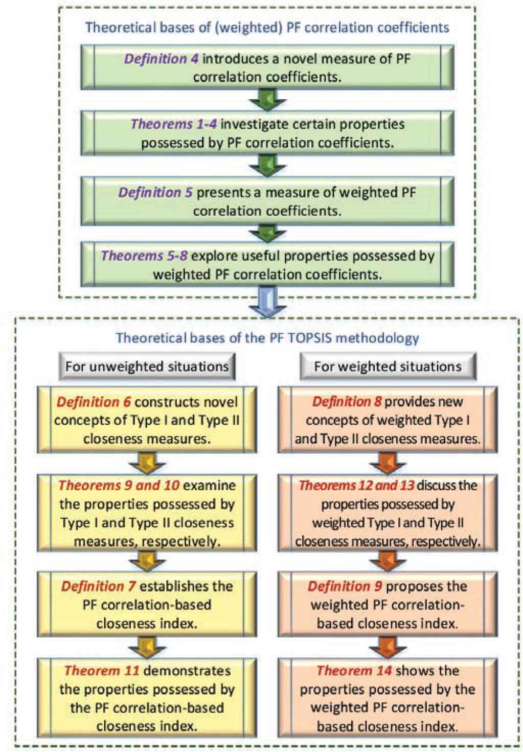
Theoretical bases of the proposed methodology.
The proposed methodology is based on the principle that the best compromise alternative should have the highest positive relationship with the positive-ideal PF solution and the lowest negative relationship with the negative-ideal PF solution. To put the assertion more concretely, the developed approach starts with the determination of new closeness measures.
Definition 6.
Let Pi, P+, and P− be the PF characteristics of an alternative zi ∈ Z, the positive-ideal PF solution z+, and the negative-ideal PF solution z−, respectively. Let MI (Pi) and MII (Pi) denote the Type I and Type II closeness measures, respectively, based on the PF correlation coefficient γ for alternative zi; they are defined as follows:
Theorem 9.
For each PF characteristic Pi in the PF decision matrix p, the Type I closeness measure MI (Pi) satisfies the following properties:
(T9.1) 0 ≤ MI (Pi) ≤ 1;
(T9.2) MI (Pi) = 1 if γ (Pi, P+) = 1;
(T9.3) MI (Pi) = 0 if γ (Pi, P−) = 1;
(T9.4) MI (P−) = 0 and MI (P+) - 1.
Proof.
For (T9.1), it is known that −1 ≤ γ (Pi, P+) ≤ 1 and −1 ≤ γ (Pi, P#) ≤ 1 based on the property in (T4.3). It follows that 0 ≤ 1 − γ (Pi, P+) ≤ 2, 0 ≤ 1 − γ (Pi, P−) ≤ 2, and 0 ≤ 2 − γ (Pi, P+) − γ Pi, P− ≤ 4. Thus, the property 0 ≤ MI (Pi) ≤ 1 can be readily inferred. For (T9.2), it is easily seen that the assumption γ (Pi, P+) = 1 results in MI (Pi) = (1 − γ (Pi, P−)) / 2 − 1 − γ (Pi, P−)) = 1. For (T9.3), when γ (Pi, P−) = 1, it can be obtained that MI (Pi) = (1 − 1) / (2 − γ (Pi, P+) − 1) = 0. For (T9.4), one has γ (P+, P+) = 1 and γ (P−, P−) = 1 according to (T4.2). Next, the properties MI (P+) = 1 and MI (P−) = 0 can be evidently inferred from (T9.2) and (T9.3), respectively. This establishes the theorem.
Furthermore, let us examine the property in (T9.2). Notice that there is a perfect positive correlation between Pi and P+ because γ (Pi, P+) = 1. The stronger the positive relationship between Pi and P+, the better the alternative zi is. It is easy to see that the Type I closeness measure in Definition 6 generates an acceptable and desirable result, that is, MI (Pi) = 1. Consider the property in (T9.3). One can also observe that there is a perfect positive correlation between Pi and P− because γ (Pi, P−) = 1. The stronger the positive relationship between Pi and P−, the worse the alternative zi is. It is clear that the Type I closeness measure in Definition 6 can produce a reasonable result, that is, MI (Pi) = 0.
Theorem 10.
For each PF characteristic Pi in the PF decision matrix p, the Type II closeness measure MII (Pi) satisfies the following properties:
(T10.1) 0 ≤ MII (Pi) ≤ 1;
(T10.2) MII (Pi) = 0 if γ (Pi, P+) = −1;
(T10.3) MII (Pi) = 1 if γ (Pi, P−) = −1;
(T10.4) MII (P−) ≤ MII (P+).
Proof.
For (T10.1), based on −1 ≤ γ (Pi, P+) ≤ 1 and −1 ≤ γ (Pi, P− ≤ 1 from (T4.3), it can be easily shown that 0 ≤ 1 + γ (Pi, P+) ≤ 2, 0 ≤ 1 + γ (Pi, P−) ≤ 2. It follows that 0 ≤ 2 + γ (Pi, P+) + γ (Pi, P−) ≤ 4. Thus, the property 0 ≤ MII (Pi) ≤ 1 can be easily acquired. For (T10.2), the assumption γ (Pi, P+) −1 indicates that MII (Pi) = (1 − 1) / (2 − 1 + γ (Pi, P−)) = 0. For (T10.3), the assumption γ (Pi, P−) = −1 leads to MII (Pi) = (1 + γ (Pi, P+)) / (2 + γ (Pi, P−) − 1) = 1. For (T10.4), based on the properties of (T4.1) and (T4.2), it is known that γ (P+, P−) = γ (P−, P+) and γ (P−, P−) = γ (P+, P+) = 1. By use of Definition 6, the following results can be obtained:
Again, let us explore the property in (T10.2). It is worth noting that there is a perfect negative correlation between Pi and P+ in case of γ (Pi, P+) = −1. The stronger the negative relationship between Pi and P+, the worse the alternative zi is. It can be observed that the Type II closeness measure in Definition 6 can yield a reasonable result, that is, MII (Pi) = 0. Next, consider the property in (T10.3). There is a perfect negative correlation between Pi and P− because γ (Pi, P−). The stronger the negative relationship between Pi and P−, the better the alternative zi is. Thus, it is clearly known that the Type II closeness measure in Definition 6 generates an acceptable result, that is, MII (Pi) = 1.
It is worth stressing that both MI (Pi) and MII (Pi) are appropriate for the specialized situations. To acquire a balanced consequence in the proposed PF TOPSIS procedure, this paper provides a comprehensive measure named as the PF correlation-based closeness index to simultaneously take into account both the Type I and Type II closeness measures.
Definition 7.
Let MI (Pi) and MII (Pi) be the Type I and Type II closeness measures, respectively, for alternative zi ∈ Z. Let ξ denote a closeness parameter, where 0 ≤ ξ ≤ 1. The PF correlation-based closeness index I(Pi) of alternative zi is defined as follows:
Theorem 11.
For each PF characteristic Pi in the PF decision matrix p, the PF correlation-based closeness index I (Pi) satisfies the following properties:
(T11.1) 0 ≤ I (Pi) ≤ 1;
(T11.2) I (Pi) = MI (Pi) if ξ = 1;
(T11.3) I (Pi) = MII (Pi) if ξ = 0;
(T11.4) I (P−) ≤ I (P+).
Proof.
(T11.1) is evident according to Definition 7 and the properties in (T9.1) and (T10.1). (T11.2) and (T11.3) are straightforward from Definition 7. For (T11.4), it is known that MI (P−) ≤ MI (P+) because MI (P−) = 0 and MI (P+) using the property in (T9.4). Moreover, one has MII (P−) ≤ MII (P+) from (T10.4). It directly follows that I (P−) ≤ I (P+). This completes the proof.
Next, consider the weighted situation in which the weight vector w = (w1, w2, ⋯, wn) is incorporated into the definitions of closeness measures.
Definition 8.
Let Pi, P+, and P− be the PF characteristics of an alternative zi ∈ Z, the positive-ideal PF solution z+, and the negative-ideal PF solution z−, respectively. Let wj be the weight of criterion cj ∈ C with wj ∈ [0, 1] and
Theorem 12.
For each PF characteristic Pi in the PF decision matrix p, the weighted Type I closeness measure
(T12.1)
(T12.2)
(T12.3)
(T12.4)
(T12.5)
Proof.
For (T12.1), by use of (T8.3), it is known that −1 ≤ γw (Pi, P+) ≤ 1 and −1 ≤ γw (Pi, P#). Thus, it is easily observed that 0 ≤ 1 − γw (Pi, P+) ≤ 2, 0 ≤ 1− γw (Pi, P−) ≤ 2, and 0 ≤ 2 − γw (Pi, P+ − γw (Pi, P−) ≤ 4. As a result, the property
Theorem 13.
For each PF characteristic Pi in the PF decision matrix p, the weighted Type II closeness measure MII (Pi) satisfies the following properties:
(T13.1)
(T13.2)
(T13.3)
(T13.4)
(T13.5)
Proof.
For (T13.1), based on −1 ≤ γw (Pi, P+) ≤ 1 and −1 ≤ γw (Pi, P−) ≤ 1 from (T8.3), it is evident that 0 ≤ 1 + γw (Pi, P+) ≤ 2, 0 ≤ 1 + γw (Pi, P−) ≤ 2, and 0 ≤ 2 + γw (Pi, P+) + γw (Pi, P−) ≤ 4. It follows that the property
Definition 9.
Let
Theorem 14.
For each PF characteristic Pi in the PF decision matrix p, the weighted PF correlation-based closeness index Iw (Pi) satisfies the following properties:
(T14.1) 0 ≤ Iw (Pi) ≤ 1;
(T14.2)
(T14.3)
(T14.4) Iw (P−) ≤ Iw (P+);
(T14.5) Iw (Pi) = I (>Pi) if w = (1/n, 1/n, ⋯, 1/n).
Proof.
(T14.1) is evident according to Definition 9 and the properties in (T12.1) and (T13.1). (T14.2) and (T14.3) are straightforward from Definition 9. For (T14.4), it is known that
Based on the proposed concepts of PF correlation coefficients, Type I and Type II closeness measures, and PF correlation-based closeness indices, this paper proposes a novel PF TOPSIS method for addressing MCDA problems involving PF information. Figure 2 illustrates the implementation procedure of the PF TOPSIS method.
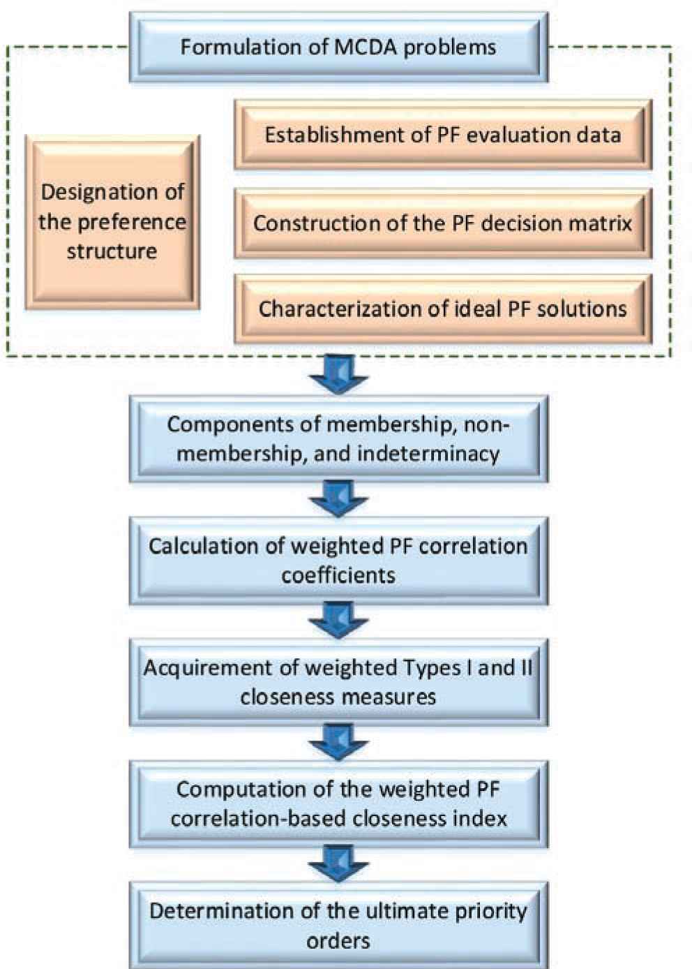
Algorithmic procedure of the proposed methodology.
The algorithmic procedure of the proposed PF TOPSIS methodology can be summarized as follows:
Step 1: Formulate an MCDA problem with the set of candidate alternatives Z = {z1, z2, ⋯, zm} and the set of evaluative criteria C = {c1, c2, ⋯, cn}, which is divided into CB and CC.
Step 2: Designate the weight vector w = (w1, w2, ⋯, wn for the n evaluative criteria. Set w = (1/n, 1/n, ⋯, 1/n in the unweighted situation.
Step 3: Establish the PF evaluative rating pij of each alternative zi ∈ Z with respect to criterion cj ∈ C.
Step 4: Form the PF decision matrix
Step 5: Identify the characteristics P+ of the positive-ideal PF solution z+ and P− of the negative-ideal PF solution z− using Equations (14) and (15), respectively.
Step 6: Compute the membership components (i.e.,
Step 7: Apply Equation (20) to derive the weighted PF correlation coefficients γw (Pi, P+) and γw (Pi, P−) between Pi and P+ and between Pi and P−, respectively, for each zi ∈ Z.
Step 8: Employ Equations (27) and (28) to compute the weighted Type I closeness measure
Step 9: Set the closeness parameter ξ, where 0 ≤ ξ ≤ 1. Calculate the weighted PF correlation-based closeness index Iw (Pi) using Equation (29) for each zi ∈ Z.
Step 10: Determine the ultimate priority orders among the m alternatives according to the descending order of the Iw (Pi) values.
6. PRACTICAL APPLICATION
This section attempts to demonstrate an illustrative application in a practical decision-making problem of hospitalization rehabilitation treatments for stroke patients with the purpose of validating the feasibility and validity of the proposed PF TOPSIS methodology. In the following, this section first describes the problem background of the medical decision concerning rehabilitation treatments for hospitalized stroke patients at acute stage.
Stroke is referred to as cerebrovascular accident. The primary cause of stroke is obstructed blood flow resulting in neurological deficits or brain hypoxia and ischemia. Stroke leads to the death or impairment of brain tissue, which may cause temporary or permanent dysfunction. According to the onset time, stroke can be divided into acute, post-acute (or sub-acute), and chronic stages. The acute stage occurs after the onset of acute stroke, and the post-acute stage occurs after patients are discharged from hospitalization for the acute phase. Finally, the chronic stage follows the post-acute stage. In particular, early rehabilitation treatment can benefit patients’ recovery of walking ability, enhance their independence in daily life, and reduce length of hospital stay. Therefore, rehabilitation treatment at the acute stage in the hospital is a crucial issue for stroke patients.
Linkou Chang Gung Memorial Hospital is located in Taoyuan City, Taiwan. The hospital’s total number of beds is approximately 3,700, and the service team comprises more than 9,000 people. Annually, the hospital provides service for 4 million outpatient clinic visits, 200,000 emergency visits, and 100,000 hospitalizations. It is the largest medical institution in Taiwan. This practical application case study explored stroke rehabilitation practices and challenges in the department of nursing of Linkou Chang Gung Memorial Hospital. Using multiple criteria as stipulated by the relevant authorities, the priorities for stroke rehabilitation treatments at the acute stage were evaluated, and the findings were used as references for clinical guidelines.
The department of nursing proposed five hospitalization rehabilitation treatments (consisting of turning over (z1), positioning (z2), passive range of motion (z3), music rehabilitation exercise (z4), and air bed (z5)) and eight evaluative criteria (consisting of pressure sore incidence (c1), aspiration pneumonia incidence (c2), arthrogryposis incidence (c3), shoulder subluxation incidence (c4), length of hospital stay (c5), degree of disability (c6), functional abilities for daily life (c7), and medical satisfaction (c8)) to assess these alternatives according to patients’ conditions. Because of the particularity of inpatient stroke rehabilitation, the medical decision-making problem of hospitalization rehabilitation treatments becomes a very complicated and ambiguous MCDA problem. To validate the effectiveness and practicability of the PF TOPSIS method, this paper employs the developed approach and techniques to assist the priority ranking of rehabilitation care services for hospitalized patients with stroke and cerebrovascular diseases.
In Step 1, the MCDA problem under study is defined by five hospitalization rehabilitation treatments and eight criteria for evaluating the alternatives. The set of candidate alternatives is denoted by Z = {z1, z2, ⋯, z5}, and the set of evaluative criteria is denoted by C = {c1, c2, ⋯, c8}, in which CB = {c1, c2, ⋯,c6} and CC = {c7, c8}.
In Step 2, based on the authority’s knowledge and expertise in the Department of Nursing at Linkou CGMH, the weight vector for the eight evaluative criteria was designated as follows: w = (0.12, 0.15, 0.17, 0.10, 0.08, 0.17, 0.14, 0.07). In Step 3, the PF evaluative rating pij of each alternative zi ∈ Z with respect to criterion cj ∈ C were established by the authority, as indicated in Table 1.
| zi | c1 | c2 | c3 | c4 | c5 | c6 | c7 | c8 |
|---|---|---|---|---|---|---|---|---|
| z1 | (0.05, 0.92) | (0.74, 0.37) | (0.51, 0.46) | (0.63, 0.57) | (0.38, 0.81) | (0.99, 0.00) | (0.13, 0.93) | (0.38, 0.68) |
| z2 | (0.12, 0.88) | (0.13, 0.87) | (0.25, 0.76) | (0.49, 0.64) | (0.76, 0.39) | (0.63, 0.60) | (0.38, 0.68) | (0.37, 0.85) |
| z3 | (0.74, 0.30) | (0.98, 0.00) | (0.13, 0.87) | (0.37, 0.73) | (0.26, 0.71) | (0.48, 0.56) | (0.52, 0.51) | (0.53, 0.55) |
| z4 | (0.87, 0.24) | (0.99, 0.00) | (0.12, 0.82) | (0.36, 0.66) | (0.24, 0.89) | (0.49, 0.57) | (0.51, 0.71) | (0.65, 0.32) |
| z5 | (0.01, 0.97) | (0.98, 0.00) | (0.86, 0.16) | (0.99, 0.01) | (0.35, 0.84) | (0.85, 0.11) | (0.13, 0.86) | (0.88, 0.21) |
Data of the PF evaluative ratings.
In Step 4, the PF decision matrix was constructed based on the PF evaluative ratings in Table 1, that is,
In Step 5, the characteristics P+ and P− of the positive- and negative-ideal PF solutions z+ and z−, respectively, were obtained as follows:
| zi | γw (Pi, P+) | γw (Pi, P−) | ||||||
|---|---|---|---|---|---|---|---|---|
| z1 | −0.4106 | 0.0553 | −0.4457 | −0.2670 | 0.4694 | 0.1351 | 0.1971 | 0.2672 |
| z2 | 0.6241 | 0.7283 | 0.5484 | 0.6336 | −0.3628 | −0.1924 | −0.3491 | −0.3015 |
| z3 | −0.2604 | 0.2067 | 0.3604 | 0.1022 | 0.0300 | −0.3781 | −0.5710 | −0.3064 |
| z4 | −0.2237 | 0.1228 | 0.2256 | 0.0416 | 0.1275 | −0.3553 | −0.6878 | −0.3052 |
| z5 | −0.4605 | −0.1008 | 0.0895 | −0.1572 | 0.6956 | 0.0629 | 0.5537 | 0.4374 |
PF, Pythagorean fuzzy.
Results of the weighted PF correlation coefficients.
In Step 9, the closeness parameter was designated as follows: ξ = 0.5. Next, the weighted PF correlation-based closeness indices were acquired as follows: Iw (P1 = 0.3665, Iw (P2) = 0.6186, Iw (P3) = 0.6432, Iw (P4) = 0.6318, and Iw (P5) = 0.4578. In Step 10, based on the descending order of these Iw (Pi) values, the ultimate priority ranking z3 ≻ z4 ≻ z2 ≻ z5 ≻ z1 was obtained as a useful decision-aiding suggestion for the MCDA problem of hospitalization rehabilitation treatments.
Furthermore, more comparative discussions of the determination results are conducted to examine the effectiveness and reasonability of the practical application. Concerning the rehabilitation treatment case, some comprehensive comparisons are depicted in Figures 3 and 4. In regard to each zi ∈ Z, the contrasts of the weighted Type I closeness measure
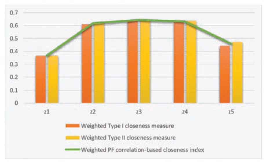
Comparison of closeness measures and PF correlation-based closeness indices.
Based on the descending orders of the
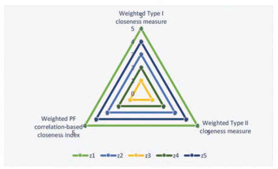
Contrast of the priority ranking orders of alternatives via
7. COMPARATIVE STUDIES
This section conducts some comparative analyses with previous researches to validate the effectiveness of the proposed approach and highlight the merits of the study.
It has to be stressed that the proposed PF TOPSIS method differs considerably from the existing TOPSIS techniques by its identification of relative closeness. As opposed to the current distance-based closeness indices, the proposed methodology employs novel concepts of PF correlations and two types of closeness measures to present the correlation-based closeness index, which is significantly different from the previous studies. Therefore, the comparative studies focus on the contrast of the obtained TOPSIS solutions based on correlation-based and distance-based closeness indices.
The comparative analyses investigate four TOPSIS techniques, consisting of the PF TOPSIS and traditional TOPSIS methods based on weighted evaluative ratings or weighted distances. As mentioned before, the current PF TOPSIS techniques presented by Gul and Ak [34], Liang and Xu [33], Liang et al. [35], Zeng et al. [32], Zhang and Xu [22], and Zhou et al. [36] employed PF distances as a separation measure to define relevant concepts of closeness indices. Referring the common TOPSIS structure based on distance-based closeness indices in these researches, this paper provides two PF TOPSIS techniques using different weighted approaches (i.e., weighted evaluative ratings and weighted distances). On the other hand, to examine the contributions and the advantages of the proposed methodology relative to the traditional TOPSIS methods, this paper converts PF evaluative ratings into crisp data via the normalized score functions. Analogously, this paper presents two traditional TOPSIS techniques based on weighted evaluative ratings and weighted distances.
The first comparative approach is the PF TOPSIS technique based on weighted evaluative ratings. For each pij (= (μij, νij)) in the PF decision matrix p, the weighted PF evaluative rating
| zi | CCw (Pi) | Iw (Pi) | |||
|---|---|---|---|---|---|
| z1 | 0.5380 | 0.4217 | 0.5463 | 0.4286 | 0.3665 |
| z2 | 0.8600 | 0.7259 | 0.8712 | 0.7480 | 0.6186 |
| z3 | 0.6156 | 0.6252 | 0.6345 | 0.6231 | 0.6432 |
| z4 | 0.5898 | 0.5858 | 0.6033 | 0.5911 | 0.6318 |
| z5 | 0.3164 | 0.3411 | 0.3287 | 0.3288 | 0.4578 |
Comparison of the obtained results.
Furthermore, a comprehensive contrast on the features and core concepts possessed by the five comparative methods is demonstrated in Table 4. The first and second comparative approaches belong to the distance-based PF TOPSIS model; moreover, the third and fourth comparative approaches belong to the distance-based traditional TOPSIS model. In contrast, the proposed methodology belongs to the correlation-based PF TOPSIS model.
| Distance-Based PF TOPSIS | Distance-Based traditional TOPSIS | Correlation-Based PF TOPSIS | ||
|---|---|---|---|---|
| Comparative approach | ||||
| PF TOPSIS based on weighted evaluative ratings | PF TOPSIS based on weighted distances | Traditional TOPSIS based on weighted evaluative ratings | Traditional TOPSIS based on weighted distances | Proposed PF TOPSIS methodology |
| Decision environment | ||||
| PF context | PF context | Certain context | Certain context | PF context |
| Separation measure | ||||
| PF distance | Weighted PF distance | Hamming distance | Weighted Hamming distance | Weighted PF correlation coefficient |
| Key index | ||||
| PF distance-based closeness index | PF distance-based closeness index | Distance-based closeness index | Distance-based closeness index | Types I & II closeness measures PF correlation-based closeness index |
PF, Pythagorean fuzzy; TOPSIS, technique for order preference by similarity to ideal solutions.
Comparison of methodological core concepts.
To provide a better view of the comparison results, this paper puts the obtained
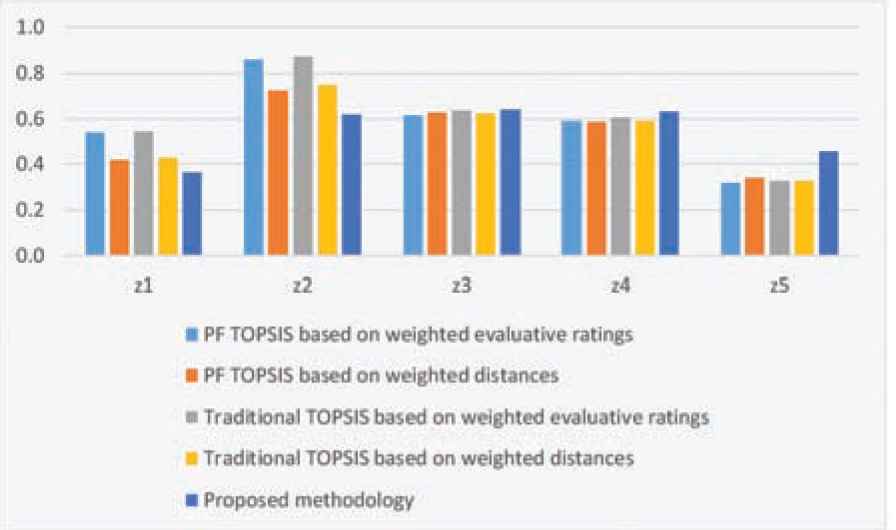
Contrast of the obtained
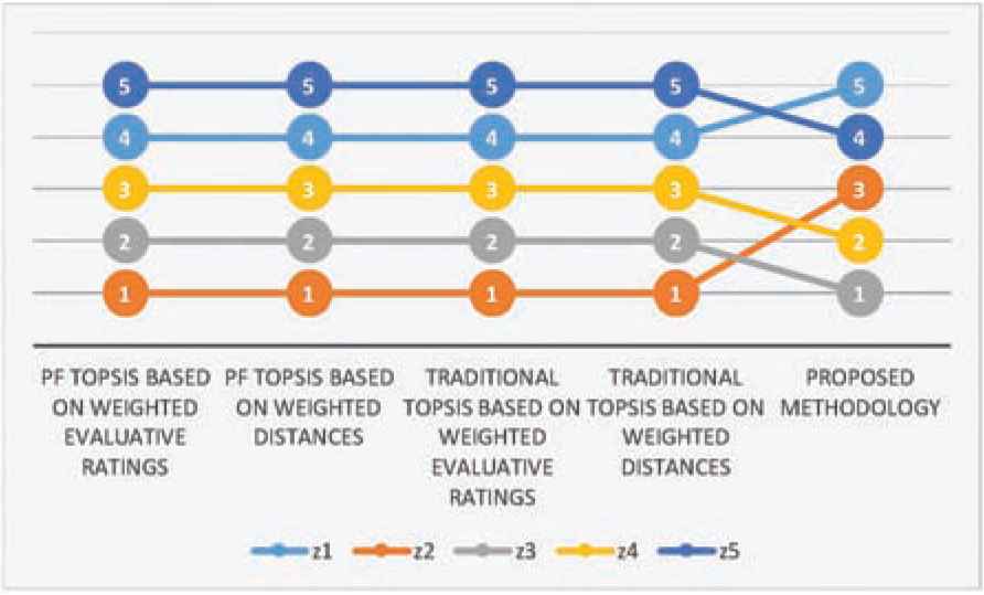
Contrast of the obtained priority ranking orders in the comparative analyses.
From Figure 6, one can find that the ranking results yielded by the two distance-based PF TOPSIS methods are identical to the results rendered by the two distance-based traditional TOPSIS methods. In contrast to the four comparative approaches mentioned above, the proposed methodology generated a different priority ranking: z3 ≻ z4 ≻ z2 ≻ z5 ≻ z1. The most prominent difference exists in the ranking orders is the alternative in first place. The alternative z2 is ranked first based on the descending order of
For the positioning treatment (z2), the following results using the modified score function were obtained:
Based on the application results of the inpatient stroke rehabilitation case, the developed PF TOPSIS method using PF correlation-based closeness indices has rationality and effectiveness to assist rehabilitation care services with cerebrovascular diseases. Moreover, the proposed PF TOPSIS methodology is highly appealing in dealing with complex PF uncertainty as it allows for greater flexibility in regard to the separation measures and traditional relative closeness by employing the new PF correlations. Furthermore, the data processing steps in the proposed algorithmic procedure are relatively simple and effective to avoid the loss of original PF uncertain information. More importantly, the proposed methodology is performed around the new concepts of weighted PF correlation coefficients and Types I and II closeness measures, while the uniformity of the core structure of classical TOPSIS is still maintained.
8. CONCLUSIONS
TOPSIS is one of the famous MCDA methods. This paper has focused on the extensions of TOPSIS applied in complicated decision environments based on PF sets. PF sets have the capability of handling more uncertainty, and hence, the PF theory has been utilized to assess and improve complex MCDA problems in this study. Based on certain useful concepts of correlation measures and PF correlation-based closeness indices, the proposed PF TOPSIS methodology would produce more accurate and robust results, as demonstrated in the practical application of inpatient stroke rehabilitation at acute stage. Furthermore, the application results can assist the rehabilitation care services for stroke patients and subsequent nursing care.
In the hospitalization rehabilitation case, the results yielded by the proposed PF TOPSIS methodology have been compared with the results generated by some previous studies, and partial differences have been observed between them. Based on the comparative discussions, the obtained results based on PF correlation-based closeness indices has shown a desirable degree of reasonability. More importantly, the combination of the core structure of TOPSIS with PF information can compensate for the lack of certainty, and allow the decision maker to arrive at an acceptable solution. Further, the proposed methodology can determine the priority ranking orders of alternatives and acquire the best compromise solution within the environment involving the objective complexity of MCDA problems and the uncertainty of human subjective judgments.
In future research, the PF TOPSIS method can be considered to be used in a multipurpose decision-making system for a wide range of applications. Concretely speaking, in the future work, the proposed methodology can be applied to address multiple criteria evaluation problems in various fields, such as logistics planning [37], situation assessment [38], credit risk evaluation [7], new product development [39], and so on. Another orientation for future research could extend the proposed methodology to deal with large-scale group decision-making problems [40, 41], bi-level decision-making problems [42, 43], tri-level decision-making problems [44, 45], and fuzzy multilevel decision-making problems [46] for enhancing theoretical value and merits of the study.
ACKNOWLEDGMENTS
The authors acknowledge the assistance of the respected editor and the anonymous referees for their insightful and constructive comments, which helped to improve the overall quality of the paper. The authors are grateful for grant funding support from the Taiwan Ministry of Science and Technology (MOST 105-2410-H-182-007-MY3) and Chang Gung Memorial Hospital (BMRP 574 and CMRPD2F0203) during the study completion.
REFERENCES
Cite this article
TY  - JOUR
AU  - Yu-Li Lin
AU  - Lun-Hui Ho
AU  - Shu-Ling Yeh
AU  - Ting-Yu Chen
PY  - 2018
DA  - 2018/11/01
TI  - A Pythagorean Fuzzy TOPSIS Method Based on Novel Correlation Measures and Its Application to Multiple Criteria Decision Analysis of Inpatient Stroke Rehabilitation
JO  - International Journal of Computational Intelligence Systems
SP  - 410
EP  - 425
VL  - 12
IS  - 1
SN  - 1875-6883
UR  - https://doi.org/10.2991/ijcis.2018.125905657
DO  - 10.2991/ijcis.2018.125905657
ID  - Lin2018
ER  -