
CPO: A Crow Particle Optimization Algorithm
Corresponding author. Email: elone.huang@nkust.edu.tw
- DOI
- 10.2991/ijcis.2018.125905658How to use a DOI?
- Keywords
- Metaheuristic algorithm; Crow search algorithm; Particle swarm optimization; Function optimization; Hybridization algorithm
- Abstract
Particle swarm optimization (PSO) is the most well known of the swarm-based intelligence algorithms and is inspired by the social behavior of bird flocking. However, the PSO algorithm converges prematurely, which rapidly decreases the population diversity, especially when approaching local optima. Recently, a new metaheuristic algorithm called the crow search algorithm (CSA) was proposed. The CSA is similar to the PSO algorithm but is based on the intelligent behavior of crows. The main concept behind the CSA is that crows store excess food in hiding places and retrieve it when needed. The primary advantage of the CSA is that it is rather simple, having just two parameters: flight length and awareness probability. Thus, the CSA can be applied to optimization problems very easily. This paper proposes a hybridization algorithm based on the PSO algorithm and CSA, known as the crow particle optimization (CPO) algorithm. The two main operators are the exchange and local search operators. It also implements a local search operator to enhance the quality of the best solutions from the two systems. Simulation results demonstrated that the CPO algorithm exhibits a significantly higher performance in terms of both fitness value and computation time compared to other algorithms.
- Copyright
- © 2019 The Authors. Published by Atlantis Press SARL.
- Open Access
- This is an open access article distributed under the CC BY-NC 4.0 license (http://creativecommons.org/licenses/by-nc/4.0/).
1. INTRODUCTION
In recent years, various metaheuristic algorithms [1] have been attracted growing interest in the optimization problems community. This kind of research is inspired by natural behavior, and it has yielded algorithms such as artificial bee colony (ABC) [2], ant colony optimization (ACO) [3], cuckoo search (CS) [4], differential evolution (DE) [5], firefly algorithm (FA) [6], gravitational searching algorithm (GSA) [7], and particle swarm optimization (PSO) [8]. In addition, various applications have been proposed for such metaheuristics algorithms in areas such as in of bioinformatics [9], clustering [10], deep learning [11], DNA fragment assembly [12], flow-shopscheduling [13], feature selection [14], geographical information systems [15], image segmentation [16], job-shop scheduling [17], power system [18], traveling salesman [19], vector quantization [20], and the water reactor problem [21].
The PSO algorithm is the most popular nature-inspired swarm-based intelligence algorithm. However, this algorithm is prone to premature convergence, especially when approaching local optima that are difficult to escape [22]. It is therefore important to maintain a sufficiently high particle diversity to avoid premature convergence. As such, several algorithms have been proposed to improve the exploration and exploitation of PSO, such as comprehensive learning PSO (CLPSO) [23], orthogonal learning PSO (OLPSO) [24], and diversity-enhanced PSO (DNSPSO) [25]. The GSA has an effective searching strategy for solving optimization problems, which is superior to and faster than the PSO algorithm. The crow search algorithm (CSA) is a recently proposed swarm-based intelligence algorithm [26] based on the intelligent behavior of crows. The main concept behind the CSA is that crows store excess food in hiding places to retrieve later when required and will attempt to cheat other crows by traveling to other positions in the search space, based on the awareness probability and flight length parameters.
Thus, we herein propose a hybridization algorithm based on the CSA and PSO algorithm, which will be referred to as the crow particle optimization (CPO) algorithm. The CPO algorithm is expected to exhibit the advantages of the CSA search strategy and the fast convergence of the PSO algorithm. The two main mechanisms of the CPO system are hybrid operation and a local search, exchanging individuals selected from the CSA and PSO systems after a specific number of iterations. Moreover, the CSA performs local searching to enhance the solution quality. The CPO process is as follows: Initially, the CPO algorithm simultaneously executes the PSO and CSA systems. Subsequently, the CPO algorithm uses center PSO (CPSO) [27] to determine the center individual of crow and the particle. The CPO algorithm then enhances the solution quality using the crossover operator [28], and finally, some individuals are selected from the PSO and CSA systems for exchange if the specific number of iterations is met. In this study, selection methods such as the roulette-wheel approach were employed [29]. Moreover, the performance of the proposed CPO algorithm was compared with those of the PSO, CSA, GSA, and PSGO algorithm using six well-known benchmark test functions. The results indicate that the CPO algorithm outperforms the others with regard to solution quality.
In this paper, the relevant background information is presented in Section 2, the proposed CPO algorithm is described in Section 3, the results of the algorithm performance tests are reported and discussed in Section 4, and the conclusions and future research outlook are given in Section 5.
2. BACKGROUND INFORMATION AND RELATED WORK
2.1. The CSA
Crows are among the most intelligent birds. Indeed, their behavior indicates a high level of intelligence only slightly below that of humans; for example, crows exhibit self-awareness in mirror tests and display tool-making abilities [30]. In fact, each crow has its own hiding place for storing food and takes precautions to protect this location from other crows, who could potentially follow the first crow to steal the stored food. CSA, which was introduced by Askazadeh [26], is a newly developed stochastic swarm-based intelligence algorithm designed to solve function optimization problems. The concepts underlying CSA are as follows:
Crows live in flocks.
They can memorize hiding-place positions.
Crows will follow one another to steal food.
They protect their hiding spaces from attackers with a probability in the interval [0, 1].
In the CSA system, the individual aggregates are described as crows. There are two main parameters for crows: the flight length fl and the awareness probability AP, respectively. The value of fl corresponds to a local search (small value) or global search (large value), and the AP controls the crow intensity (small value) or diversity (large value). These crows are randomly generated at certain positions by the CSA. The fitness values are computed and the position of each crow in the current population is updated using Equation (1). The position of crows i in iteration t, which provides a potential solution for N crows, is defined as follows:
The current solution for each crow is then updated according to one of two cases. In the first case, it is assumed that crow c does not know that crow i is in pursuit. In the second case, it is assumed that crow c knows that crow i is in pursuit. The updated position for each crow is computed using Equation (2):
The CSA algorithm is described in Figure 1.
| Step | Description |
|---|---|
| 1. | Initialize all crow positions with randomization |
| 2. | Initialize memories of all crows |
| 3. | Obtain fitness values for all crows |
| 4. | Obtain memories of all crows |
| 5. | Update all crow positions according to Equation 2 |
| 6. | Repeat Steps 35 until termination criterion is reached |
| 7. | Output the best solution |
Standard crow search algorithm (CSA).
2.2. Particle Swarm Optimization
The PSO algorithm, which was introduced by Kennedy and Eberhart [8, 31] is a stochastic swarm-based intelligence algorithm that is a widely known because of its efficient searching strategy. Similar to the genetic algorithm (GA), PSO is inspired by the collective behavior of schools of fish or bird flocks. In the PSO algorithm, the positions and velocities of N particles in the d-dimensional space offer randomly initialized solutions. The solution of particle i in iteration t is as given by Equation (3). The current solution of each particle is then updated with regard to the local and global optima, which are computed using Equations (4) and (5), respectively.
The PSO algorithm is detailed in Figure 2.
| Step | Description |
|---|---|
| 1. | Initialize solution with randomization. |
| 2. | Obtain fitness values for all particles |
| 3. | Obtain personal best solution for each particle |
| 4. | Obtain global best solution for all particles |
| 5. | Update positions and velocities of all particles according to Equations 4 and 5 |
| 6. | Repeat Steps 2–5 until maximum iteration is reached |
| 7. | Output best solution |
Standard PSO algorithm.
2.3. Center Particle Swarm Optimization
Liu et al. [32] proposed an improved PSO approach known as center particle swam optimization (CPSO). In this study, we employed the concepts to improve the PSO and CSA systems. The main concept behind CPSO is that a population of N particles is considered, and their positions represent potential solutions. After the position values are updated for N − 1 particles, a center particle cp is added to the population, as follows Equation (6):
| Step | Description |
|---|---|
| 1. | Initialize solution with a randomization |
| 2. | Calculate center particle cp based on all particles to Equation (6) |
| 3. | Obtain fitness values for all particles |
| 4. | Obtain personal best solution for each particle |
| 5. | Obtain global best solution for all particles |
| 6. | Update positions and velocities of all particles according to Equations (4) and (5) |
| 7. | Repeat Steps 2–6 until maximum iteration is reached |
| 8. | Output best solution |
Center particle swarm optimization (CPSO) algorithm [32].
3. PROPOSED CPO ALGORITHM
We herein present our proposed CPO algorithm, which couples the PSO and CSA systems. More specifically, CPO involves simultaneously executing the PSO and CSA systems and guiding the solution toward the global optimum using the CPSO algorithm. Some individuals are selected from the PSO and CSA systems using selection approaches and are exchanged following the processing of a specific number of iterations. Finally, a local search operator is used to improve the solution quality.
3.1. Individual Velocity
During successive iterations, the solution space is searched for each particle and its solution is updated using Equation (4). Oscillations in the PSO algorithm are controlled by a time-varying maximum velocity Vmax. The velocity thresholds are given by the expressions presented in the literature [33], as shown in Equations (7) and (8):
3.2. Hybrid Operator
A hybrid operator is called at specific iterations. Some individuals are selected from the CSA and PSO systems and exchanged using the selection approaches. In this study, random selection was employed along with the roulette-wheel approach [29] with probabilities depending on the fitness values. The roulette-wheel approach is expressed as Equation (9):
An example of the hybrid operator is shown in Figure 4. In the CSA system, the random number is 0.23 and is located in the region Cl, while the random number of the PSO algorithm is 0.30, located in the region P2. Thus, in the roulette-wheel operator, the particle number C1 and agent number P2 are selected for exchange between the two systems.
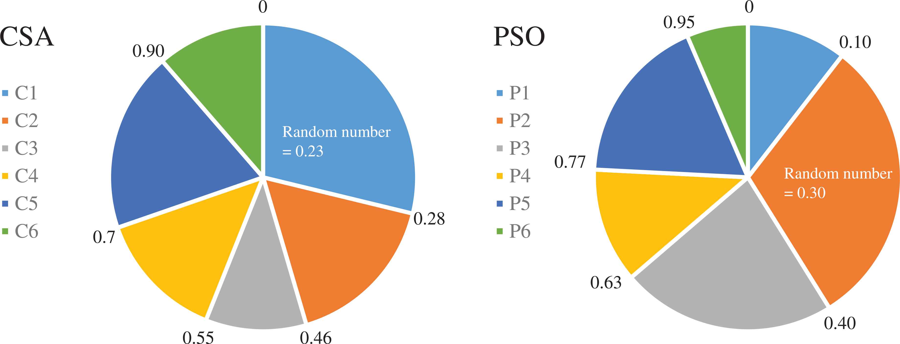
Example of the hybrid operator.
3.3. Local Search Operator
The local search operator proposed in this study is similar to the DE crossover operator [28]. Denoting crow c as the best of individual crow,
An example of the local operator is shown in Figure 5. Iteration t, assuming the PSO solutions for each dimension are 2.3, 1.5, 0.5, 0.8, 5.5, and 1.7, the CSA solutions for each corresponding dimension are 3.7, 0.3, 1.6, 0.1, 3.7, and 4.8, respectively. According to Equation (10), the new best solution is 2.3, 0.3, 0.5, 0.1, 3.7, and 1.7, respectively.
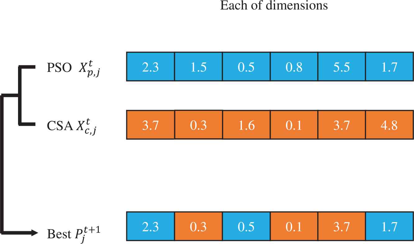
Example of the local search operator.
3.4. Summary of CPO Algorithm
Figure 6 shows the procedure of the proposed CPO algorithm. In the initial step, each crow (particle) is generated at random. Upon implementation of the CPSO algorithm to determine a central crow or particle, the CPO algorithm simultaneously executes the CSA and PSO algorithm to update the solutions of the two systems. After a specific number of iterations and exchange of a crow and a particle, it becomes necessary to trigger the hybrid operator. Finally, the quality of the best solution is improved using the local search operator.
| Step | Description |
|---|---|
| 1. | Initialize each agent with a randomized position and velocity in the CSA and PSO |
| 2. | Obtain the center crow and particle according to Equation 6 |
| 3. | Execute CSA process according to Figure 1 |
| 4. | Execute PSO process according to Figure 2 |
| 5. | Rim the local operator to increase the best solutions among both systems |
| 6. | If specific iteration is reached, implement hybrid operator |
| 7. | If terminal criterion is not met, repeat Steps 2–6 |
| 8. | Best solution is found |
Proposed crow particle optimization (CPO) algorithm.
4. EXPERIMENT AND RESULTS
4.1. Environment Setting
Numerous simulations were conducted to evaluate the performance of the proposed CPO algorithm. All simulation results were obtained using a computer with an i7-6700 3.40-GHz Intel CPU and 8GB of main memory running on Microsoft Windows 7. All programming was implemented using Java language.
4.2. Benchmark Functions
The six benchmark test functions used in our experiments (namely the Sphere, Rosenbrocks, Ackley, Griewanks, Schwefel, and Rastrigin functions) are described in Table 1 [23]. In this case, d is the function dimensions, which was set to 10 for the purpose of study. The optimal solution of each benchmark function is 0d.
| Test Function | Formula | Solution Space | Optimal Value |
|---|---|---|---|
| Sphere | [−100, 100]d | 0 | |
| Rosenbrocks | [−2.048, 2.048]d | 0 | |
| Ackley | [−32.768, 32.768]d | 0 | |
| Griewanks | [−600, 600]d | 0 | |
| Schwefel | [−10, 10]d | 0 | |
| Rastrigin | [−5.12, 5.12]d | 0 |
Test functions.
4.3. Parameter Settings
The basic parameter settings are listed in Table 2. All experimental results were collected from 30 independent runs, each involving 2000 iterations.
| Algorithm | Parameter | Value |
|---|---|---|
| CSA | Number of crows | 20 |
| Flight length fl | 1.5 | |
| Awareness probability AP | 0.05 | |
| PSO | Number of particles | 20 |
| Inertia ω | 0.9 to 0.4 | |
| c1, c2 | 1.4 | |
| h | 0.05 | |
| α | 0.01 | |
| CPO | Number of individuals | 20 |
CSA, crow search algorithm; PSO, particle swarm optimization; CPO, crow particle optimization.
Parameter settings for proposed algorithm.
4.4. Comparison of Selection Approaches
Two different selection strategies were compared to determine the optimal strategy for selection of the individuals from the CSA and PSO systems. More specifically, the roulette wheel and random selection methods were considered, and the exchange iterations and individuals were set to 20 and 5, respectively. The simulated best solutions and average best fitness values (labeled Best and Average, respectively), as well as the average computation times (S) tavg are summarized in Table 3. In terms of the best fitness value, the roulette-wheel operator outperformed the random selection operator for test functions f2, f3, f4, f5, and f6. Similarly, for the average fitness value, the roulette-wheel operator outperformed the random selection operator for functions f1, f2, f4, and f6. Both approaches had almost identical computation times. Overall, the roulette-wheel approach was superior to the random selection strategy in the context of this study.
| Strategy | f1 | f2 | f3 | f4 | f5 | f6 | |
|---|---|---|---|---|---|---|---|
| Roulette-wheel | Best | 5.15E-56 | 1.12E+00 | 3.55E-15 | 7.39E-3 | 7.32E-43 | 9.96E-01 |
| Average | 3.52E-20 | 4.49E+00 | 1.74E-10 | 6.70E-2 | 2.85E-13 | 3.55E+00 | |
| tavg(s) | 0.03 | 0.03 | 0.08 | 0.07 | 0.03 | 0.07 | |
| Random selection | Best | 2.86E-87 | 1.82E+00 | 7.10E-15 | 3.90E-2 | 5.40E-32 | 1.98E+00 |
| Average | 8.73E-20 | 4.76E+00 | 8.27E-11 | 9.10E-2 | 2.58E-13 | 4.62E+00 | |
| tavg(s) | 0.03 | 0.03 | 0.08 | 0.07 | 0.03 | 0.07 |
Comparison of different selection operators of the crow particle optimization (CPO) algorithm for d = 10.
4.5. Comparison of CPO With Difference Variants
As mentioned in the previous subsection, the roulette-wheel operator was found to provide the best solutions, so this operator was selected for use in the remaining experiments. Several variants of the CPO algorithm were compared in the subsequent simulations, for which the number of iterations and individuals exchanged among the composite algorithms were varied, as detailed in Table 4. Variant 1 was used for the comparison of selection approaches reported in the previous subsection. In Variant 1, two individuals were exchanged between the two systems every 20 iterations, whereas for Variant 3, 10 individuals were exchanged between the two systems every 20 iterations. In the majority of cases, d was set to 10, the number of iterations was 2000, and the number of simulations was 30.
| Variants | Specific Iterations | Specific Individuals |
|---|---|---|
| 1 | 20 | 5 |
| 2 | 20 | 2 |
| 3 | 20 | 10 |
| 4 | 50 | 5 |
| 5 | 75 | 5 |
| 6 | 75 | 2 |
Parameters for six variants of proposed algorithm
The simulated best solutions and average best fitness values (labeled Best and Average, respectively), and the average computation times tavg are summarized in Table 5. In terms of best fitness, CPO Variant 4 outperformed all other variants for test functions f3, f4, and f6; Variant 2 outperformed the other variants for functions f2, and f5; and Variant 5 yielded the best solution for f1. The highest average fitness values for functions f1, f2, f5, and f6 were yielded by Variants 6, Variants 2, Variants 1, and Variants 5, respectively, while Variant 4 was the best performer for functions f3 and f4. In contrast, the computation times were comparable among all variants. We therefore concluded that Variant 4 yielded the average case of better solutions among the variants examined herein.
| Variants | f1 | f2 | f3 | f4 | f5 | f6 | |
|---|---|---|---|---|---|---|---|
| 1 | Best | 1.70E-70 | 1.35E+00 | 3.55E-15 | 0.00E+00 | 5.34E-43 | 1.99E+00 |
| Average | 7.18E-20 | 4.68E+00 | 2.33E-10 | 6.34E-02 | 2.27E-13 | 4.02E+00 | |
| tavg(s) | 0.03 | 0.03 | 0.07 | 0.06 | 0.03 | 0.06 | |
| 2 | Best | 4.28E-68 | 2.26E+00 | 3.55E-15 | 7.40E-03 | 2.24E-50 | 9.95E-01 |
| Average | 6.36E-20 | 5.00E+00 | 2.33E-10 | 6.47E-02 | 4.08E-13 | 4.22E+00 | |
| tavg(s) | 0.03 | 0.03 | 0.07 | 0.06 | 0.03 | 0.06 | |
| 3 | Best | 1.43E-60 | 3.84E-01 | 3.55E-15 | 7.40E-03 | 7.71E-52 | 9.95E-01 |
| Average | 7.40E-19 | 4.24E+00 | 2.17E-10 | 5.93E-02 | 5.40E-13 | 3.36E+00 | |
| tavg(s) | 0.03 | 0.03 | 0.07 | 0.06 | 0.03 | 0.06 | |
| 4 | Best | 5.45E-49 | 9.56E-01 | 3.55E-15 | 0.00E+00 | 1.81E-26 | 8.15E-01 |
| Average | 1.41E-19 | 4.66E+00 | 1.05E-10 | 5.38E-02 | 5.97E-13 | 4.62E+00 | |
| tavg(s) | 0.03 | 0.03 | 0.07 | 0.06 | 0.03 | 0.06 | |
| 5 | Best | 1.96E-96 | 6.60E-01 | 2.42E-12 | 0.00E+00 | 6.13E-38 | 9.95E-01 |
| Average | 4.57E-19 | 4.78E+00 | 2.02E-10 | 6.32E-02 | 4.41E-13 | 3.31E+00 | |
| tavg(s) | 0.03 | 0.03 | 0.07 | 0.06 | 0.03 | 0.06 | |
| 6 | Best | 1.64E-64 | 1.35E+00 | 3.55E-15 | 7.40E-03 | 3.54E-46 | 9.95E-01 |
| Average | 5.52E-20 | 4.75E+00 | 1.24E-10 | 7.21E-02 | 3.69E-13 | 3.55E+00 | |
| tavg(s) | 0.03 | 0.03 | 0.07 | 0.06 | 0.03 | 0.06 |
Comparison of different variants of the crow particle optimization (CPO) algorithm for d = 10.
To present the previous experimental results more clearly, the data from Table 5 are depicted visually Figure 7. The x-axis shows the different variants, and the y-axis shows the log values of the best and average fitness values for each test function. In addition, we divided the six functions into two groups due to f2 and f4 having different value ranges, with some fitness values larger than 1.
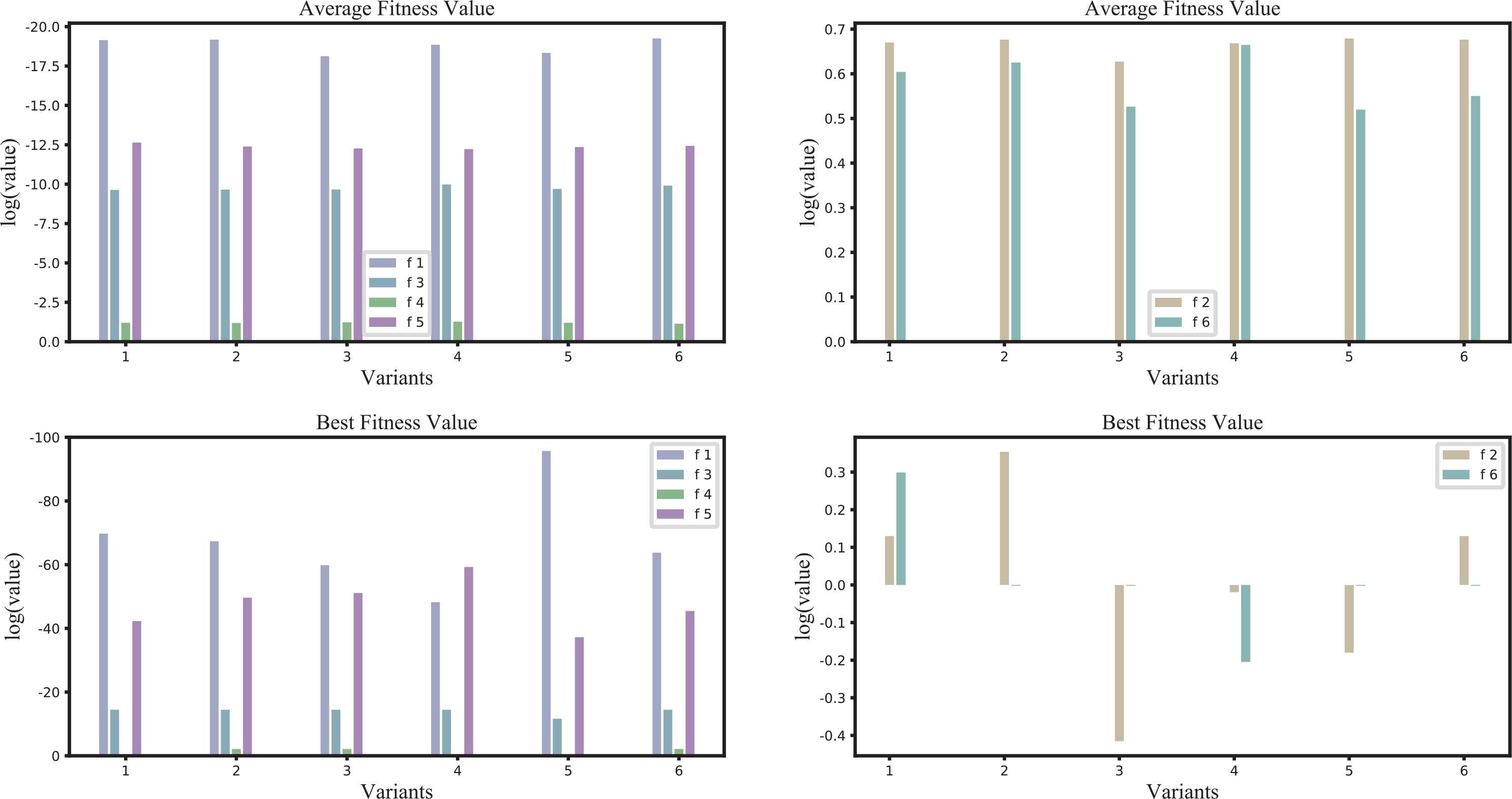
Comparison of the results for different variants.
4.6. Comparison of the CPO With PSO, CSA, GSA, and PSGO Algorithm
As described in the previous subsection, Variant 4 of the CPO algorithm provided the best solutions. Therefore, CPO was employed using the parameters of Variant 4 for comparison with the CSA [26], PSO [8], GSA [7], and PSGO [34] algorithm for 2000 iterations of the six benchmark test functions. The settings employed for all CSA and PSO algorithms were as described for the CPO, as detailed in Table 2.
Table 6 gives the best solution and average best fitness values (labeled Best and Average, respectively), as well as the average computation time(s) tavg for each simulation. In terms of the best fitness value, the PSO algorithm provided the best fitness for functions f1 and f2, whereas the CPO algorithm outperformed the other algorithms for f3, f4, f5, and f6. For the average fitness values, the GSA provided the average best fitness for function f1, while the CPO algorithm outperformed the other algorithms for f2, f4, f5, and f6. Furthermore, the computational time for the CPO algorithm was only 50% that of for the GSA, and the computational times of CPO and PSGO were comparable.
| Algorithm | Fitness Value | f1 | f2 | f3 | f4 | f5 | f6 |
|---|---|---|---|---|---|---|---|
| CPO | Best | 3.87E-54 | 8.07E-01 | 3.55E-15 | 5.52E-03 | 1.20E-32 | 9.95E-01 |
| Average | 1.60E-21 | 4.62E+00 | 2.25E-11 | 2.56E-02 | 1.59E-13 | 3.87E+00 | |
| tavg | 0.03 | 0.03 | 0.07 | 0.06 | 0.03 | 0.06 | |
| CSA | Best | 4.07E-18 | 3.07E+00 | 4.70E-10 | 1.48E-02 | 1.64E-10 | 1.99E+00 |
| Average | 1.5E-9 | 4.70E+00 | 3.37E-09 | 4.04E-02 | 4.11E-10 | 5.03E+00 | |
| tavg | 0.01 | 0.01 | 0.03 | 0.03 | 0.01 | 0.03 | |
| PSO | Best | 2.86E-87 | 4.37E-02 | 3.55E-15 | 3.94E-02 | 8.23E-50 | 2.98E+00 |
| Average | 1.27E-04 | 7.99E+00 | 6.03E-06 | 2.84E-01 | 6.83E-01 | 8.64E+00 | |
| tavg | 0.02 | 0.02 | 0.04 | 0.04 | 0.02 | 0.03 | |
| GSA | Best | 3.55E-28 | 5.21E+00 | 3.20E-14 | 0.00E+00 | 3.77E-14 | 1.99E+00 |
| Average | 1.09E-25 | 5.61E+00 | 4.78E-13 | 2.08E-01 | 3.02E-12 | 6.70E+00 | |
| tavg | 0.09 | 0.10 | 0.15 | 0.11 | 0.05 | 0.11 | |
| PSGO | Best | 6.26E-06 | 7.64E+00 | 2.66E-04 | 2.21E-02 | 8.46E-05 | 2.15E+00 |
| Average | 1.61E-05 | 8.38E+00 | 1.48E-03 | 5.33E-02 | 2.45E-04 | 6.13E+00 | |
| tavg | 0.04 | 0.04 | 0.07 | 0.06 | 0.04 | 0.06 |
PSO, particle swarm optimization; CSA, crow search algorithm; CPO, crow particle optimization; GSA, gravitational searching algorithm.
Comparison of CPO with CSA, PSO, GSA, and PSGO.
To present previous experimental result more clearly, the data from Table 6 depicted visually in Figure 8. The x-axis shows the different variants, and the y-axis shows the log values of the best and average fitness values for each test function. In addition, we divided the six functions into two groups due to f2 and f4 having different value ranges, with some fitness values are larger than 1.
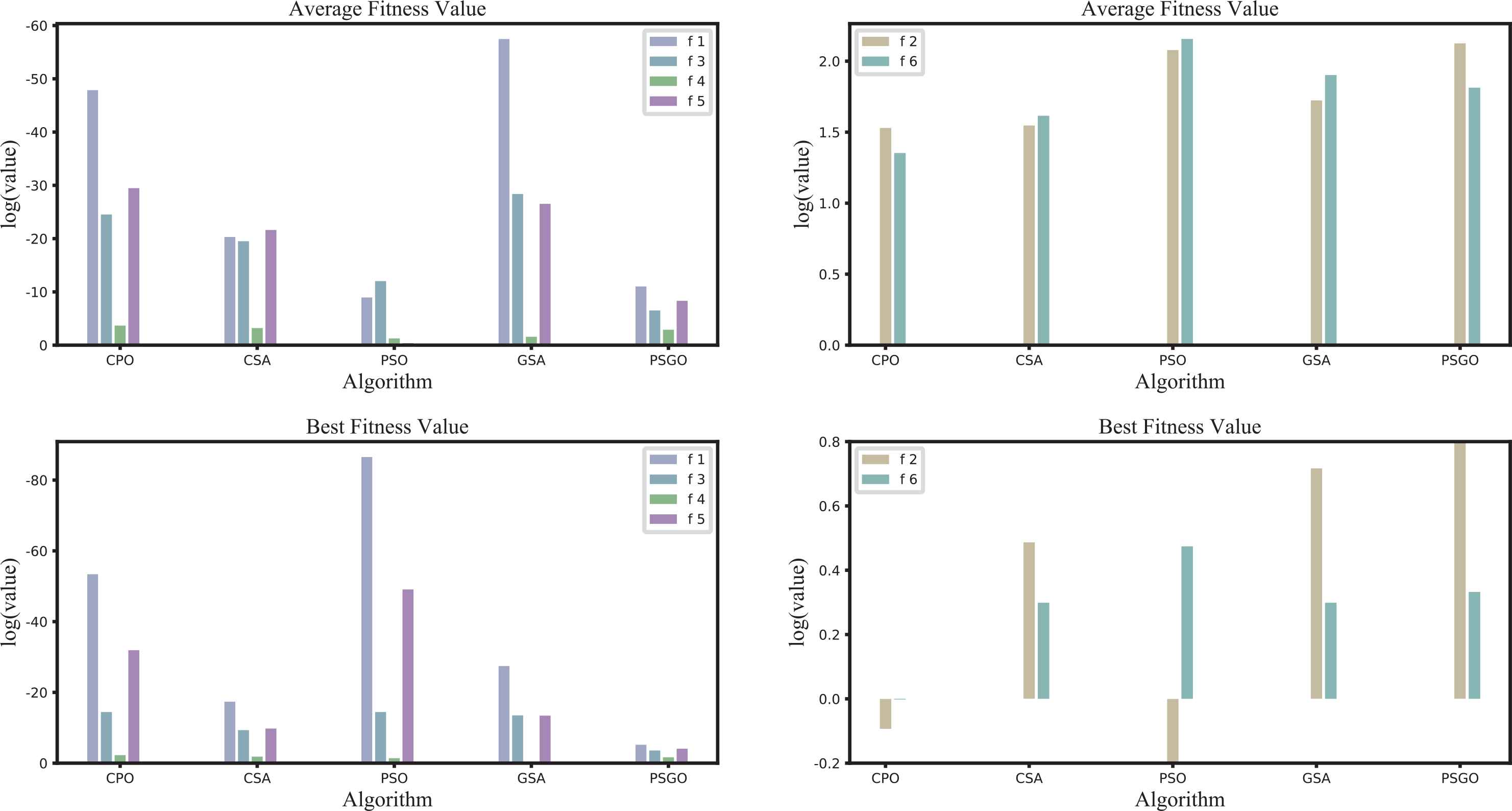
Comparison of the results for all specified algorithms.
4.7. Convergence Rates
Finally, the convergence rates of the CSA, PSO, GSA, PSGO, and CPO were investigated. For each benchmark function from f1 to f6, the convergence rates of the average best fitness values for 30 runs of 2000 iterations, are presented in Figure 9.
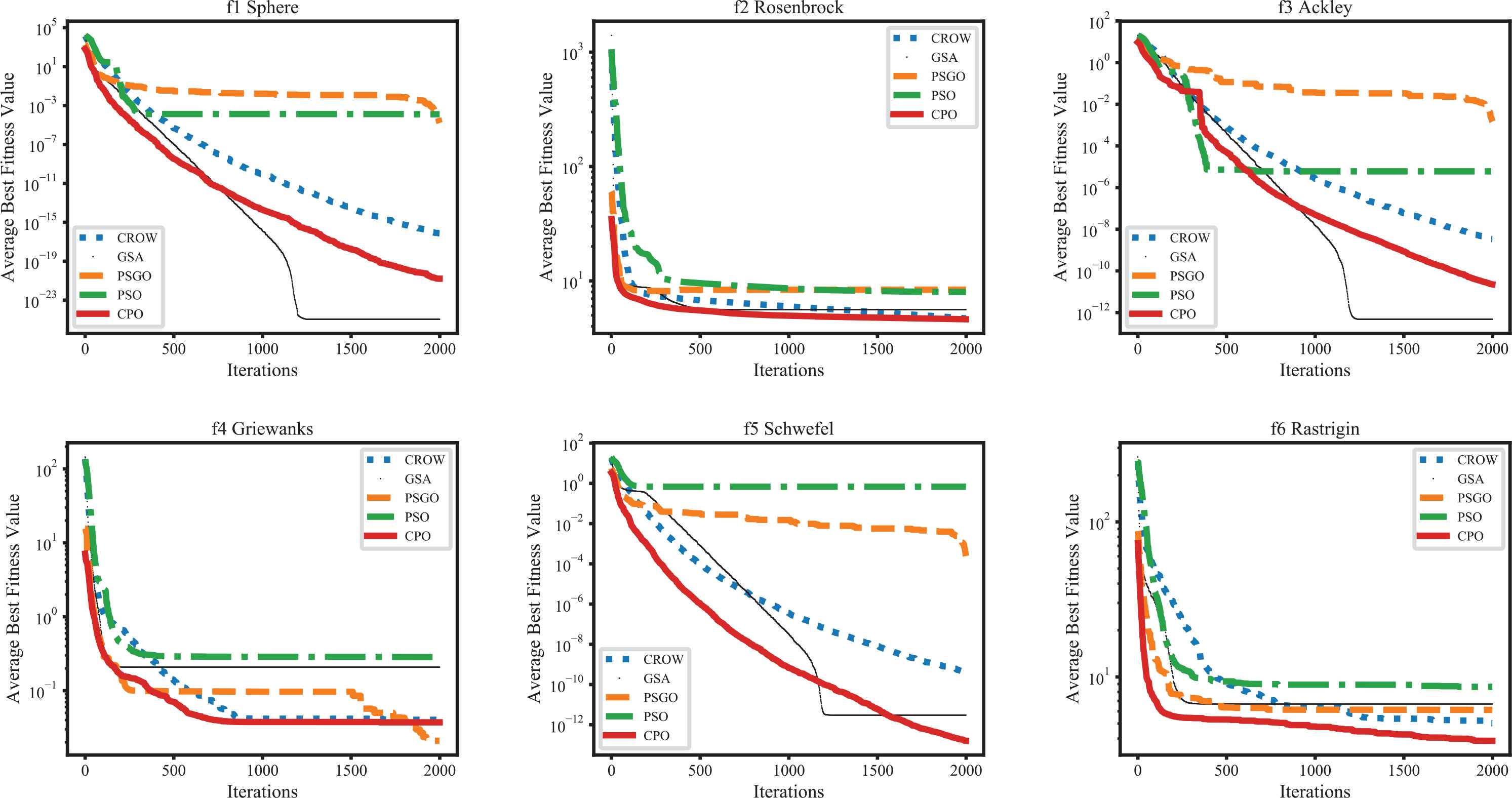
Comparisons of the convergence rates for all specified algorithms over 2,000 iterations.
As indicated clearly by the obtained results, a relationship exists between the convergence speed and the best solution. Indeed, the GSA outperformed the other algorithms in terms of the convergence rate for f1 and f3, and the GSA is superior to the CPO algorithm for f1 and f3, but the convergence line for the CPO algorithm is still decreasing. The PSO algorithm exhibits the highest convergence speed for f4, f5, and f6. Comparing the results of the CPO algorithm and CSA, it is apparent that CPO is more effective for all test functions. Comparing the results of CPO and PSGO indicates that CPO can outperform PSGO. In summary, the proposed CPO algorithm can yield the best results with the lowest convergence speed. In contrast, the results for the PSO algorithm are unstable, as this algorithm can yield the best solution for one simulation but the worst solution when averaged over all simulations.
4.8. Scalability of CPO and GSA
As apparent from the results, there is a relationship between the convergence speed and best solution. The GSA outperformed the other algorithms in terms of convergence rate for f1 and f3. However, although the GSA can get a better solution than CPO in f1 and f3, the result is in convergence status, and the convergence line of CPO is still decreasing. Thus, in this section, to verify that CPO can provide better solutions than the GSA in large numbers of iterations, we present a comparison of the CPO algorithm with the GSA for scalability using 10,000 iterations. The convergence rates of the average best fitness values for 30 runs, each consisting of 10,000 iterations, are presented in Figure 10.
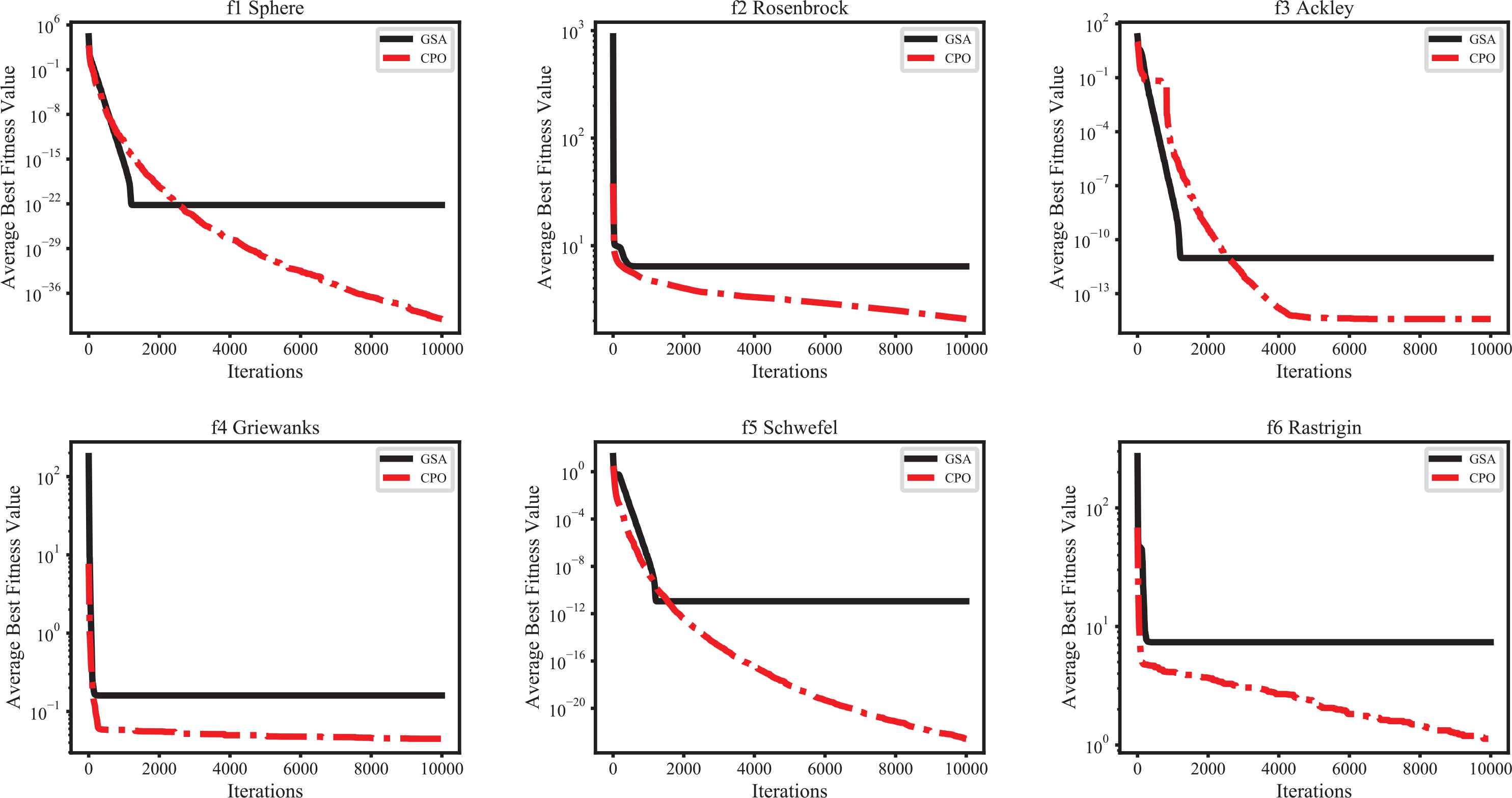
Comparison of convergence rates between CPO and GSA for f1 to f6.
The GSA yields better solutions using fewer than 2000 iterations, but CPO provides better solutions in terms of convergence rate for f1 to f6 when compared with the GSA for more than 2000 iterations. In summary, the results confirm that the proposed CPO algorithm can yield the lowest convergence speed.
5. CONCLUSIONS AND FUTURE WORK
To improve the global search performance of the CSA, we proposed a CPO algorithm to solve function optimization problems. In this case, the CPO algorithm simultaneously executes the PSO and CSA systems, before using the CPSO algorithm to generate the center individual. Subsequently, in specific iterations, some individuals from the PSO and CSA systems are selected for exchange using the roulette-wheel method. Finally, the local search operator is fine-tuned to yield the best solutions, which include the best individuals among those of the CSA and PSO systems. This CPO approach exhibits significantly better performance than the existing algorithms in terms of the average fitness values and computation times for six benchmark test functions. Future studies will focus on our investigation into application of the CPO algorithm to nondeterministic polynomial hard combinatorial problems such as clustering issues and medical image processing, as well as diversity enhancement of the CPO system to avoid fast convergence.
ACKNOWLEDGMENTS
This work was supported in part by the Ministry of Science and Technology, Taiwan, R.O.C., under grants MOST 107-2218-E-992 -303.
REFERENCES
Cite this article
TY  - JOUR
AU  - Ko-Wei Huang
AU  - Ze-Xue Wu
PY  - 2019
DA  - 2019/02/06
TI  - CPO: A Crow Particle Optimization Algorithm
JO  - International Journal of Computational Intelligence Systems
SP  - 426
EP  - 435
VL  - 12
IS  - 1
SN  - 1875-6883
UR  - https://doi.org/10.2991/ijcis.2018.125905658
DO  - 10.2991/ijcis.2018.125905658
ID  - Huang2019
ER  -