
AEkNN: An AutoEncoder kNN–Based Classifier With Built-in Dimensionality Reduction
Corresponding author. Email: fpulgar@ujaen.es
- DOI
- 10.2991/ijcis.2018.125905686How to use a DOI?
- Keywords
- kNN; Deep learning; Autoencoders; Dimensionality reduction; High dimensionality
- Abstract
High dimensionality tends to be a challenge for most machine learning tasks, including classification. There are different classification methodologies, of which instance-based learning is one. One of the best known members of this family is the k-nearest neighbors (kNNs) algorithm. Its strategy relies on searching a set of nearest instances. In high-dimensional spaces, the distances between examples lose significance. Therefore, kNN, in the same way as many other classifiers, tends to worsen its performance as the number of input variables grows. In this study, AEkNN, a new kNN-based algorithm with built-in dimensionality reduction, is presented. Aiming to obtain a new representation of the data, having a lower dimensionality but with more informational features, AEkNN internally uses autoencoders. From this new vector of features the computed distances should be more significant, thus providing a way to choose better neighbors. An experimental evaluation of the new proposal is conducted, analyzing several configurations and comparing them against the original kNN algorithm and classical dimensionality reduction methods. The obtained conclusions demonstrate that AEkNN offers better results in predictive and runtime performance.
- Copyright
- © 2019 The Authors. Published by Atlantis Press SARL.
- Open Access
- This is an open access article distributed under the CC BY-NC 4.0 license (http://creativecommons.org/licenses/by-nc/4.0/).
1. INTRODUCTION
Classification is a well-known task within the area of machine learning [1]. The main objective of a classifier is to find a way to predict the label to be assigned to new data patterns. To do so, usually a model is created from previously labeled data. In traditional classification, each example has a single label. Different algorithms have been proposed in order to address this work. One of the classic methodologies is instance-based learning (IBL) [2]. Essentially, this methodology is based on local information provided by the training instances, instead of constructing a global model from the whole data. The algorithms belonging to this family are relatively simple, however they have shown to obtain very good results in tackling the classification problem. A traditional example of such an algorithm is k-nearest neighbors (kNNs) [3].
The different IBL approaches, including the kNN algorithm [4], have difficulties when faced with high-dimensional datasets. These datasets are made of samples which contain a large number of features. In particular, the kNN algorithm presents problems when calculating distances in high-dimensional spaces. The main reason is that distances are less significant as the number of dimensions increases, tending to equate [4]. This effect is one of the causes of the curse of dimensionality, which occurs when working with high-dimensional data [5]. Another consequence that emerges in this context is the Hughes phenomenon. This fact implies that the predictive performance of a classifier decreases as the number of features of the dataset grows, keeping the number of examples constant [6]. In other words, more instances would be needed to maintain the same level of performance.
Several approaches have been proposed for to deal with the dimensionality reduction task. Recently, a few proposals based on deep learning (DL) [7, 8] have obtained good results while tackling this problem. The rise of these techniques is produced by the good performance that DL models have had in many research areas, such as computer vision, automatic speech processing, or audio and music recognition. In particular, autoencoders (AEs) are DL networks offering good results due to their architecture and operation [9–11].
High dimensionality is usually mitigated by transforming the original input space into a lower-dimensional one. In this paper an instance-based algorithm, that internally generates a reduced set of features, is proposed. Its objective is to obtain a better IBL method, able to deal with high-dimensional data.
The present study introduces AEkNN, a kNN-based algorithm with built-in dimensionality reduction. AEkNN projects the training patterns into a lower-dimensional space, relying on an AE to do so. The goal is to perform the classification using new features of higher quality and lower dimensionality [9]. This approach is experimentally evaluated, and a comparison between AEkNN and the kNN algorithm is performed considering predictive performance and execution time. The results obtained demonstrate that AEkNN offers better results in both metrics. In addition, AEkNN is compared with other traditional dimensionality reduction algorithms. This comparison offers an idea of the behavior of the AEkNN algorithm when facing the task of dimensionality reduction.
An important aspect of the AEkNN algorithm that must be highlighted is that it performs a transformation of the features of the input data, in contrast to other traditional feature selection algorithms that perform a simple selection of the most significant features. AEkNN performs this transformation taking into account all the characteristics of the input data, although not all will have the same weight in the new generated space.
In short, AEkNN combines two reference methods, kNN and AE, in order to take advantage of kNN in classification and reduce the effects of high dimensionality by means of AE. Summarizing, the main contributions of this study are 1. the design of a new classification algorithm, AEkNN, which combines an efficient dimensionality reduction mechanism with a popular classification method, 2. an analysis of the AEkNN operating parameters that allows selection of the best algorithm configuration, 3. an experimental demonstration of the improvement that AEkNN achieves with respect to the kNN algorithm, 4. an experimental comparison between the use of an AE for dimensionality reduction with respect to other classical methods such as principal components analysis (PCA) and linear discriminant analysis (LDA), 5. a set of guidelines for the reader when using the AEkNN algorithm, and 6. results on the use of AEkNN in real cases.
This paper is organized as follows: In Section 2 some details about the kNN algorithm, DL techniques, and AEs are provided. Section 3 describes relevant studies related to this proposal, focused on tackling the problem of dimensionality reduction in kNN. In Section 4, the proposed AEkNN algorithm is introduced. Section 5 defines the experimental framework, as well as the different results obtained from the experimentation. Finally, Section 6 provides the overall conclusions.
2. PRELIMINARIES
In general terms, machine learning is a subfield of Artificial Intelligence whose aim is to develop algorithms and techniques able to generalize behaviors from information supplied as examples. Classification is one of the tasks performed in the data mining phase. It is a predictive task that usually develops through supervised learning methods [12]. Its purpose is to predict, based on previously labeled data, the class to assign to future unlabeled patterns.
Several issues can emerge while designing a classifier, with some of them related to high dimensionality. According to the Hughes phenomenon [6], the predictive performance of a classifier decreases as the number of features increases, provided that the number of training instances is constant. Another phenomenon that particularly affects IBL methods is the curse of dimensionality. IBL algorithms are based on the similarity of individuals, calculating distances between them [2]. These distances tend to lose significance as dimensionality grows.
AEkNN, the algorithm proposed in this study, is a kNN-based classification method designed to deal with high-dimensional data. This section outlines the essential concepts AEkNN is founded on, such as nearest neighbors classification, DL techniques, and AEs. The kNN algorithm is discussed in Subsection 2.1, while DL and AEs are briefly described in Subsections 2.2 and 2.3.
2.1. The kNN Algorithm
kNN is a nonparametric algorithm developed to deal with classification and regression tasks [3]. In classification, kNN predicts the class for new instances using the information provided by the kNNs, so that the assigned class will be the most common among them. Figure 1 shows a very simple example of how kNN works with different k values. As can be seen, the prediction obtained with k = 3 would be B, with k = 5 would be A and with k = 11 would be A.
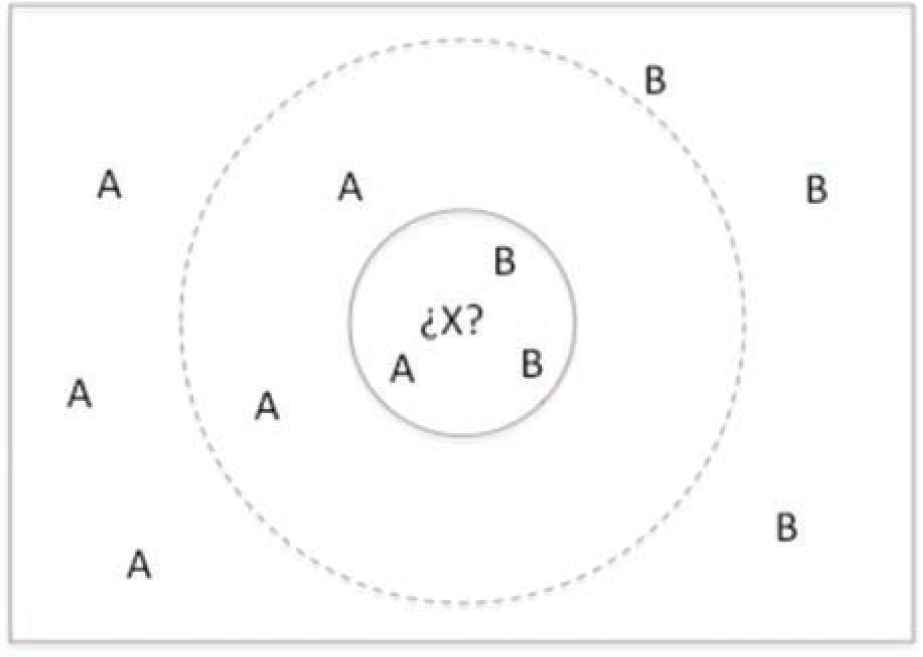
kNN algorithm in a bidimensional space.
An important feature of this algorithm is that it does not build a model for accomplishing the prediction task. Usually, no work is done until an unlabeled data pattern is encountered, thus the denomination of lazy approach [13]. Once the instance to be classified is given, the information provided by its kNNs [14] is used as explained above.
One of kNN’s main issues is its behavior with datasets which have a high-dimensional input space. Nowadays, the generation of information is growing in all fields of research. Therefore, when dealing with many real problems it is necessary to use increasingly larger datasets. This fact implies the need to deal with the problem of high-dimensional space when working with machine learning algorithms.
In particular, kNN is affected by the high dimensionality due to the loss of significance of traditional distances as the dimensionality of the data increases [4]. This fact occurs because the distances from the farthest points and closest to any data pattern do not increase as fast as the minimum of the two. This is obviously a problem, since it indicates a poor discrimination of the closest and farthest points with respect to the reference pattern [15]. In such a high-dimensional space distances between individuals tend to be the same. As a consequence similarity-/distance-based algorithms, such as kNN, usually do not offer adequate results.
However, kNN is very popular since it has a good performance, uses few resources, and it is relatively simple [16, 17]. The objective of this proposal is to present an algorithm that combines the advantages of kNN in classification with DL models to reduce dimensionality.
2.2. Deep Learning
DL [7] arises with the objective of extracting higher-level representations of the analyzed data. In other words, the main goal of DL-based techniques is to learn complex representations of data. The main lines of research in this area are intended to define different data representations and create models to learn them [18].
As the name suggests, models based on DL are developed as multilayered (deep) architectures, which are used to map the relationships between features in the data (inputs) and the expected result (outputs) [19, 20]. Most DL algorithms learn multiple levels of representations, producing a hierarchy of concepts. These levels correspond to different degrees of abstraction. The following are some of the main advantages of DL:
These models can handle a large number of variables and generate new features as part of the algorithm itself, not as an external step [7].
Provides performance improvements in terms of time needed to accomplish feature engineering, one of the most time-consuming tasks [19].
Achieves much better results than other methods based on traditional techniques [21] when dealing with problems in certain fields, such as image, speech recognition, or malware detection.
DL-based models have a high capacity of adaptation for facing new problems [20, 22].
Recently, several new methods [7, 8, 23] founded on the good results produced by DL have been published. Some of them are focused on certain areas, such as image processing and voice recognition [21]. Other DL-based proposals have been satisfactorily applied in disparate areas, gaining advantage over prior techniques [7]. Due to the great impact of DL-based techniques, as well as the impressive results they usually offer, new challenges are also emerging in new research lines [8].
There are two main reasons behind the rise of DL techniques, the large amount of data currently available and the increase in processing power. In this context, different DL architectures have been developed: AEs (Section 2.3), convolutional neural networks [24, 25], long short-term memory [26], recurrent neural networks [27], gated recurrent unit [28], deep Boltzmann machines [29], deep stacking networks [30], deep coding networks [31], deep recurrent encoder [32], deep belief networks [33], among others [7, 20].
DL models have been widely used to perform classification tasks obtaining good results [21]. However, the objective of this proposal is not to perform the classification directly with these models, but use them to the dimensionality reduction ask.
The goal of the present study is to obtain higher-level representations of the data but with a reduced dimensionality. One of the dimensionality reduction DL-based techniques that has achieved good results is the use of AEs [34]. An AE is an artificial neural network whose purpose is to reproduce the input into the output, in order to generate a compressed representation of the original information [20]. Section 2.3 describes this technique in detail.
2.3. Autoencoders
An AE is an artificial neural network able to learn new information encodings through unsupervised learning [9]. AEs are trained to learn an internal representation that allows reproduction the input into the output through a series of hidden layers. The goal is to produce a more compressed representation of the original information in the hidden layers, so that it can be used in other tasks. AEs are typically used for dimensionality reduction tasks owing to their characteristics and performance [10, 11, 35]. Therefore, this is the reason to choose AEs in this paper.
The most basic structure of an AE is very similar to that of a multilayer perceptron. An AE is a feedforward neural network without cycles, so the information always goes in the same direction. AEs are typically formed by a series of layers: an input layer, a series of hidden layers, and an output layer, with the units in each layer connected to those in the next. The main characteristic of AEs is that the output has the same number of nodes as the input, since the goal is to reproduce the latter in the former throughout the learning process [20].
Two parts can be distinguished in an AE, the encoder and the decoder. The first is made up of the input layer and the first half of hidden layers. The second is composed of the second half of hidden layers and the output layer. This is the architecture shown in Figure 2. As can be seen, the structure of an AE always is symmetrical.
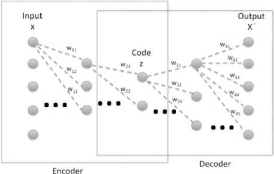
Architecture of autoencoder with three hidden layers.
The encoder and decoder parts in an AE can be defined as functions ω (Equation (1)) and β (Equation (2)), so that:
Equation (3) corresponds to the compression function, for which an encoded input representation is obtained. Here, γ1 is an activation function such as a rectified linear unit or a sigmoid function.
The next step is to decode the new representation z to obtain x’, in the same way as x was projected into z, by means of a weight vector W’ and a bias parameter b’. Equation (4) corresponds to the decoder part, where the AE reconstructs the input from the information contained in the hidden layer.
During the training process, the AE tries to reduce the reconstruction error. This operation consists of back-propagating the obtained error through the network, and then modifying the weights to minimize any error. Algorithm 1 shows the pseudocode of this process.
Algorithm 1 AE training algorithm’s pseudocode.
Inputs:
TrainData ▷ Train Data
1: ▷ For each training instance:
2: for each instance in TrainData do
3: ▷ Do a feed-forward through AE to obtain output:
4: newCod ← feedForwardAE(aeModel, instance)
5: ▷ Calculate error:
6: error ← calculateError(newCod, instance)
7: ▷ Backpropagate the error through AE and perform weight update:
8: aeModel ← backpropagateError(error)
9: end for
Learning a representation that allows reproducing the input into the output could seem useless at first sight, but in this case the output is not of interest. Instead, the concern is in the new representation of the inputs learned in the hidden layers. Such new codification is really interesting, because it can have very useful features [19]. The hidden layers learn a higher-level representation of the original data, which can be extracted and used in independent processes.
Depending on the number of units the hidden layers have, two types of AEs can be distinguished:
Those whose hidden layer has fewer units than the input and output layers. This type of AE is called undercomplete. Its main objective is to force the network to learn a compressed representation of the input, extracting new, higher-level features.
Those whose hidden layer has more units than the input and output layers. This type of AE is called overcomplete. The main problem in this case is that the network can learn to copy the input to the output without learning anything useful, so when it is necessary to obtain an enlarged representation of the input it is necessary to use other tools to prevent this problem.
In conclusion, AEs are a very suitable tool for generating a new lower-dimensional input space consisting of higher-level features. AEs have obtained good results in performing this task. This is the main reason to choose this technique to design the AEkNN algorithm described later. However, it is important to note that there are other methods of dimensionality reduction that produce good results, such as denoising AEs [36], restricted Boltzmann machines (RBMs) [37], or sparse coding [38]. The objective of this proposal is to present an algorithm that hybridizes kNN with AEs. This establishes a baseline that allows supporting studies with more complex methods.
3. DIMENSIONALITY REDUCTION APPROACHES
In this section, an exploration of previous studies related to the proposal made in this paper is carried out. Subsection 3.1 introduces classical proposals to tackle the dimensionality reduction problem. Some approaches for facing the dimensionality reduction task for kNN are outlined in Subsection 3.2.
In automatic learning, dimensionality reduction is the process aimed to decrease the number of considered variables, by obtaining a subset of main features. Usually two different dimensionality reduction methods are considered:
Feature selection [39], where the subset of the initial features that provides more useful information is chosen. The final features have no transformation in the process.
Feature extraction [40], where the process constructs from the initial features a set of new ones providing more useful and nonredundant information, facilitating the next steps in machine learning and in some cases improving understanding by humans.
3.1. Classical Proposals for Dimensionality Reduction
Most dimensionality reduction techniques can be grouped into two categories, linear and nonlinear approaches [41]. Below some representative proposals found in the literature, which can be considered as traditional methods, are shown.
Commonly, classical proposals for dimensionality reduction were developed using linear techniques, such as the following:
PCA [42] is a well-known solution for dimensionality reduction. Its objective is to obtain the lower-dimensional space where the data are embedded. In particular, the process starts from a series of correlated variables and converts them into a set of uncorrelated linear variables. The variables obtained are known as principal components, and their number is less than or equal to the original variables. Often, the internal structure extracted in this process reflects the variance of the data used.
Factors analysis [43] is based on the idea that the data can be grouped according to their correlations, that is, variables with a high correlation will be within the same group and variables with low correlation will be in different groups. Thus, each group represents a factor in the observed correlations. The potential factors plus the terms error are linearly combined to model the input variables. The objective of factor analysis is to look for independent dimensions.
Classical scaling [44] consists in grouping the data according to their similarity level. An algorithm of this type aims to place all data in an N-dimensional space where the distances are maintained as much as possible.
Despite their popularity, classical linear solutions for dimensionality reduction present the problem that they cannot correctly handle complex nonlinear data [41]. For this reason, nonlinear proposals for dimensionality reduction arose. A compilation of these is presented in [45, 46]. Some of these techniques are Isomap [47], Maximum Variance Unfolding [48], diffusion maps [49], manifold charting [41], among others. These techniques allow working correctly with complex nonlinear data. This is an advantage when working with real data, which are usually of this type.
3.2. Proposals for Dimensionality Reduction in kNN
There are different proposals trying to deal with the problems of kNN when working with high-dimensional data. In this section, some of them are collected:
A method for computing distances for kNN is presented in [50]. The proposed algorithm performs a partition of the total data set. Subsequently, a reference value for each partition made is assigned. Grouping the data in different partitions allows to obtain a space of smaller dimensionality where the distances between the reference points are more significant. The method depends on the division of the data performed and the selection of the reference.
The experimentation presented in [50] shows an improvement in efficiency. However, the methodology used can be affected by high-dimensional data. In this type of scenario, the distances between the data are less significant, and therefore, the groupings can include instances with very different features. Thus, relevant information can be lost during the process. Likewise, performance depends on the choice of the representative element of each subset, that is, a bad choice can influence the final results.
The authors of [51] analyze the curse of dimensionality phenomenon, which states that in high-dimensional spaces the distances between the data points become almost equal. The objective is to investigate when the different methods proposed reach their limits. To do this, they perform an experiment in which different methods are compared with each other. In particular, it is found that the kNN algorithm begins to worsen the results when the space exceeds eight dimensions. A proposed solution is to adapt the calculation of distances to high-dimensional spaces. However, this approach does not consider a transformation of the initial data to a lower-dimensional space.
One of the most important aspects of this study is that it demonstrates how dimensionality affects the kNN method. However, the proposed solution consists of a modification in the calculation of distances. In this way, the consequences of high dimensionality can be alleviated, but solutions must be found that make it possible to reduce the input space. The fundamental reason is that the dimensionality will continue to increase in the future and other methods, like AEkNN, can be better adapted to the new data.
The proposal in [52] is a kNN-based method called kMkNN, whose objective is to improve the search of the nearest neighbors in a high-dimensional space. This problem is approached from another point of view, with the goal of accelerating the computation of distances between elements without modifying the input space. To do this, kMkNN relies on k-means clustering and the triangular inequality. The study shows a comparison with the original kNN algorithm where it is demonstrated that kMkNN works better considering the execution time, although it is not as effective when predictive performance is taken into account.
The main problem with the kMkNN method is that it makes a grouping of examples in different clusters. In this way, in spaces of high dimensionality where distances are less significant, instances with different characteristics can be included in the same cluster. This implies a significant loss of relevant information, which translates into worse predictive results. However, the execution time is reduced when clusters are used to classify. Despite the improvement in time, kMkNN method is not a good option as predictive performance is adversely affected.
A new aspect related to the curse of dimensionality phenomenon, occurring while working with the kNN algorithm, is explored in [53]. It refers to the number of times that a particular element appears as the closest neighbor of the rest of elements. The main objective of the study is to examine the origins of this phenomenon as well as how it can affect dimensionality reduction methods. The authors analyze this phenomenon and some of its effects on kNN classification, providing a foundation which allows making different proposals aimed to mitigate these effects.
The proposed solution is based on finding hubs, that is, popular elements that effectively represent a set of close neighbors. The fundamental problem of this approach is that it does not consider all the input data, but uses a representative for different instances. In this way, relevant information may be removed from the process. Furthermore, the loss of useful information can increase as the dimensionality increases, since the distances between elements are less significant.
In [15], the problem of finding the nearest neighbors in a high-dimensional space is analyzed. This is a difficult problem both from the point of view of performance and the quality of results. In this study, a new search approach is proposed, where the most relevant dimensions are selected according to certain quality criteria. Thus, the different dimensions are not treated in the same way. This can be seen as an extraction of characteristics according to a particular criterion. Finally, an algorithm based on the previous approach, which tackles the problem of the nearest neighbor, is proposed.
The proposal made in this study is based on the selection of the most relevant input features. This choice is made according to different preestablished criteria, which implies discarding some input features. Therefore, this process does not take into account all the input characteristics. In certain cases, this fact may not be relevant. However, in other cases, important information may be lost when discarding input features. This situation has greater effect in spaces of high dimensionality. Therefore, proposals that generate new features by considering all the input information could provide better results.
A method called DNet-kNN is presented in [54]. It consists in a nonlinear feature mapping based on Deep Neural Network, aiming to improve classification by kNN. DNet-kNN relies on RBMs to perform the mapping of characteristics. RBMs are another type of DL network [55]. The study offers a solution to the problem of high-dimensional data when using kNN by combining this traditional classifier with DL-based techniques. The experimentation carried out proves that DNet-kNN improves the results of the classical kNN.
The main strength of this algorithm is the use of DL models to carry out dimensionality reduction. In addition, DNet-kNN combine DL model with kNN to improve predictive performance. However, it is based on RBM and requires pretraining the model to generate good results. This implies a previous phase, separated from the proposed algorithm. Another negative aspect is that the experimentation is only based on two datasets (digits and letters) and does not include datasets from other areas, such as medical.
In conclusion, different proposals have arisen to analyze and try to address the problems of IBL algorithms when they have to deal with high-dimensional data. These methods are affected by the curse of dimensionality, which raises the need to find new approaches. Among the previous proposals, there is none that presents a hybrid method based on IBL that incorporates the reduction of dimensionality intrinsically. In addition, there are not many proposals that obtains improvements both in predictive performance as well as in execution time. The present study is aimed to fulfilling these aspects.
4. AEKNN: AN AUTOENCODER KNN-BASED CLASSIFIER WITH BUILT-IN DIMENSIONALITY REDUCTION
Once the main foundations behind our proposed algorithm have been described, this section presents AEkNN. It is an instance-based algorithm with a built-in dimensionality reduction method, performed with DL techniques, in particular by means of AEs.
4.1. AEkNN Foundations
As mentioned, high dimensionality is an obstacle for most classification algorithms. This problem is more noticeable while working with distance-based methods, given that as the number of variables increases these distances are less significant [6, 51]. In such situation an IBL method could lose effectiveness, since the distances between individuals are equated. As a consequence of this problem, different methods which are able to reduce its effects have been proposed. Some of them have been previously listed in Section 3.2.
AEkNN is a new approach in the same direction, introducing the use of AEs to address the problem of high dimensionality. The structure and performance of this type of neural networks makes it suitable for this task. As explained above, AEs are trained to reproduce the input into the output, through a series of hidden layers. Usually, the central layer in AEs has fewer units than the input and output layers. Therefore, this bottleneck forces the network to learn a more compact and higher-level representation of the information. The coding produced by this central layer can be extracted and used as the new set of features in the classification stage. In this sense, there are different studies demonstrating that better results are obtained with AEs than with traditional methods, such PCA or multidimensional scaling [10, 41]. Also, there are studies analyzing the use of AEs from different perspectives, either focusing on the training of the network and its parameters [56] or on the relationship between the data when building the model [35].
AEkNN is an instance-based algorithm designed to address classification with a high number of variables. It starts working with an N-dimensional space X that is projected into an M-dimensional space Z, with M < N. This way M new features, presumably of higher level than the initial ones, are obtained. Once the new representation of the input data is generated, it is possible to get more representative distances. To estimate the output, the algorithm uses the distances between each test example and the training ones but based on the M higher-level features. Thus, the drawbacks of high-dimensional data in distances computation can be significantly reduced. As can be seen, AEkNN is a nonlazy instance-based algorithm. It starts by generating the model in charge of producing the new features, unlike the lazy methods that do not have a learning stage or model. AEkNN allows enhancement of predictive performance, as well as obtaining improvements in execution time, when working with data which have a large number of features.
4.2. Method Description
AEkNN consists of two fundamental phases. Firstly, the learning stage is carried out using the training data to generate the AE model that enables production of a new encoding of the data. Secondly, the classification step is performed. It uses the model generated in the first phase to obtain the new representation of the test data and, later, the class for each instance is estimated based on nearest neighbors. Algorithm 2 shows the pseudocode of AEkNN, which is discussed in detail below, while Figure 3 shows a general representation of the algorithm process.
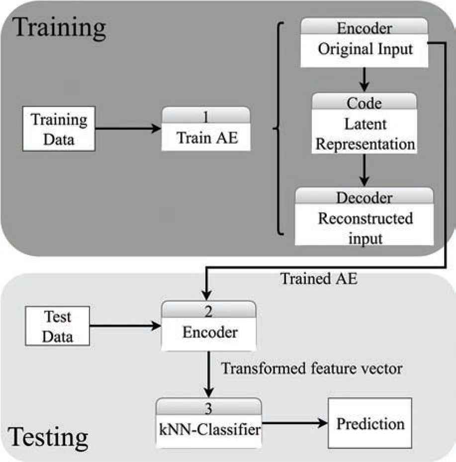
Method description.
Algorithm 2 AEkNN algorithm’s pseudocode.
Inputs:
TrainData ▷ Train Data
TestData ▷Test Data
PPL ▷Percentage per layer
k ▷ Number of nearest neighbors
1: ▷ Training phase:
2: modelData ← TrainData
3: aeModel ← ()
4: for each layer in PPL do
5: sizeLayer ← getSizeLayer(modelData, layer)
6: aeLayer ← getAELayer(modelData, sizeLayer)
7: modelData ← applyAELayer(aeLayer, modelData)
8: aeModel ← addAEModel(aeModel, aeLayer)
9: end for
10: ▷ Classification phase:
11: result ← classification(TrainData, TestData, k, aeModel)
12: return result
13:
14: function
15: aeLayer ← initializeAE(modelData, sizeLayer)
16: for each instance in modelData do
17: output ← feedForwardAE(aeLayer, instance)
18: error ← calculateDeviation(instance, outPut)
19: aeLayer ← updateWeightsAE(aeLayer, error)
20: end for
21: return aeLayer
22: end function
23:
24: function CLASSIFICATION(TrainData, TestData, k, aeModel)
25: error ← 0
26: for each instance in TestData do
27: newCod ← feedForwardAE(aeModel, instance)
28: output ← distanceBased(newCod, k, TrainData)
29: if outPut ! = realOutPut(instance) then
30: error ← error + 1
31: end if
32: end for
33: result ← error / size(TestData)
34: return result
35: end function
The inputs to the algorithm are TrainData and TestData, the train and test data to be processed, k, the number of neighbors, and PPL, the percentage of elements per layer (PPL). This latter parameter sets the structure of the AE, that is, the number of layers and elements per layer. It is a vector made of as many items as hidden layers are desired in the AE, each indicating the percentage of units in that layer with respect to the number of input features. In Section 5, different configurations are analyzed to find the one that offers the best results.
The algorithm is divided into two parts. The first part of the code (lines 2–9) corresponds to the training phase of AEkNN. The second part (lines 11–12) refers to the classification phase. During training AEkNN focuses on learning a new representation of the data. This is done through an AE, using the training data to learn the weights linking the AE’s units. This is a process that has to be repeated for each layer in the AE, stated by the number of elements in the PPL parameter. This loop performs several tasks:
In line 5 the function getSizeLayer is used to obtain the number of units in the layer. This value will depend on the number of characteristics of the training set (TrainData) and the percentage applied to the corresponding layer, which is established by the PPL parameter.
The function getAELayer (called in line 6 and defined in line 14) retrieves a layer of the AE model. The layer obtains a new representation of the data given as first parameter (modelData). The number of units in the AE layer generated in this iteration will be given by the second parameter (sizeLayer). Firstly, the AE is initialized with the corresponding structure (line 15). The number of units in the hidden layer is given by the variable computed in the previous step, and the weights are randomly initialized. Secondly, for each training instance the following steps take place:
The AE is used to obtain the output for the given instance (line 17).
The deviation of the given output with respect to the actual one is calculated (line 18).
The weights of the network are updated according to the obtained error (line 19).
Finally, the generated AE layer is returned (line 21).
The function applyAELayer (line 7) obtains a new representation of the data given as second parameter (modelData). To do this, the previously generated AE layer, represented by the first parameter (aeLayer), is used.
The last step consists in adding the AE layer generated in the current iteration to the complete AE model (line 8).
During classification (lines 11–12) the function classification is used (lines 24–35). The class for the test instances given as the first parameter (TestData) is predicted. The process performed internally in this function is to transform each test instance using the AE model generated in the training phase (aeModel), producing a new instance, which is more compact and representative. (line 27). This new set of features is used to predict a class with a classifier based on distances, using for each new example its kNNs (line 28). Finally, this function returns the error rate (result) for the total set of test instances (line 33). As can be seen, classification is conducted in a lower-dimensional space, mitigating the problems associated with a high number of variables.
At this point, it should be clarified that the update of weights (lines 16–20) is carried out using mini-batch gradient descent [57]. This is a variation of the gradient descent algorithm that splits the training dataset into small batches that are used to calculate the model error and update the model coefficients. The reason for using this technique is its improved performance when dealing with large dataset.
From the previous description is can be inferred how AEkNN accomplish the objective of addressing classification with high-dimensional data. On the one hand, aiming to reduce the effects of working with a large number of variables, AEs have been used to transform such data into a lower-dimensional space. On the other hand, the classification phase is founded on the advantages of IBL.
4.3. AEkNN Contributions with Respect to Previous Proposals
AEkNN presents significant differences with previous proposals that tackled kNN while dealing with high-dimensional spaces. In this section, the objective is to highlight the main contributions of AEkNN with respect the proposals analyzed in Section 3.2:
AEkNN is an IBL method that integrates dimensionality reduction. For this reason, it does not need a preprocessing phase where the size of the input space is reduced. This is an improvement over classical kNN and the method presented in [50], which requires a previous grouping of the data to select the most representative patterns.
AEkNN performs a fusion of features that implies the generation of new features from the original input space. This allows incorporation of the most relevant information of the different characteristics. This implies advantages over the proposal made in [15], where it selects a specific number of original features, discarding the rest, as well as the information that they can provide. Likewise, it is an advantage over the proposals [50, 53] where the elements are grouped into subsets and a representative element is selected.
The parametrization of AEkNN allows to perform different degrees of dimensionality reduction, according to the characteristics of the problem and the needs of the user. This implies being able to work with a dataset with a very large dimensionality. In this sense, the authors of [51] propose a modification on the calculation of distances. However, this study does not verify its proposal with really large datasets, where the effects of high dimensionality are very significant.
AEkNN has been proposed to improve both the predictive performance and the execution time of kNN with high-dimensional data. However, the proposal made in [52] focuses only on the improvement in time, while not effective when analyzing the predictive performance.
The development of AEkNN aims to provide a useful algorithm for different types of datasets. Therefore, the experimentation carried out in this study covers data of different nature. Nevertheless, the proposal made in [54] is based on analyzing only two dataset. In this way, the development of the model is limited to focusing on the properties of specific data.
In this section, an analysis of the contributions of the AEkNN method with respect to other previous proposals has been performed. In order to justify the behavior of the method, extensive experimentation has been designed. To do this, Section 5 analyzes the performance of AEkNN.
5. EXPERIMENTAL STUDY
In order to demonstrate the improvements provided by AEkNN, an experimental study was conducted. It has been structured into three steps, all of them using the same set of datasets:
The objective of the first phase is to determine how the PPL parameter in AEkNN influences the obtained results. For this purpose, classification results for all considered configurations are compared in Subsection 5.2. At the end, the value of the PPL parameter that offers the best results is selected.
The second phase aims to verify whether AEkNN with the selected configuration improves the results provided by the classic kNN algorithm. In Subsection 5.3, the results of both algorithms are compared.
The third phase of the experimentation aims to assess the competitiveness of AEkNN against traditional dimensionality reduction algorithms, in particular, PCA and LDA. In Subsection 5.4, the results of the three algorithms are compared.
Subsection 5.1 describes the experimental framework and the following subsections present the results and their analysis.
5.1. Experimental Framework
The conducted experimentation aims to show the benefits of AEkNN over a set of datasets with different characteristics. Their traits are shown in Table 1. The datasets’ origin is shown in the column named Ref. For all executions, datasets are given as input to the algorithms applying a 2 × 5 folds cross validation scheme.
| Dataset | Samples | Number of Features | Classes | Type | Ref |
|---|---|---|---|---|---|
| image | 2310 | 19 | 7 | Real | [58] |
| drive | 58509 | 48 | 11 | Real | [58] |
| coil2000 | 9822 | 85 | 2 | Integer | [59] |
| dota | 102944 | 116 | 2 | Real | [58] |
| nomao | 1970 | 118 | 2 | Real | [58] |
| batch | 13910 | 128 | 6 | Real | [60] |
| musk | 6598 | 168 | 2 | Integer | [58] |
| semeion | 1593 | 256 | 10 | Integer | [58] |
| madelon | 2000 | 500 | 2 | Real | [61] |
| hapt | 10929 | 561 | 12 | Real | [62] |
| isolet | 7797 | 617 | 26 | Real | [63] |
| mnist | 70000 | 784 | 10 | Integer | [64] |
| microv1 | 360 | 1300 | 10 | Real | [58] |
| microv2 | 571 | 1300 | 20 | Real | [58] |
Characteristics of the datasets used in the experimentation.
In both phases of experimentation, the value of k for the classifier kNN and for AEkNN will be 5, since it is the recommended value in the related literature. In addition, to compare classification results it was necessary to compute several evaluation measures. In this experimentation, Accuracy (5), F-Score (6), and area under the ROC curve (AUC) (9) were used.
Accuracy (5) is the proportion of true results among the total number of cases examined.
F-Score is the harmonic mean of Precision (7) and Recall (8), considering Precision as the proportions of positive results that are true positive results and Recall as the proportion of positives that are correctly identified as such. These measures are defined by the Equations (6–8):
Finally, AUC is the probability that a classifier will rank a randomly chosen positive instance higher than a randomly chosen negative one. AUC is given by Equation 9:
The significance of results obtained in this experimentation is verified by appropriate statistical tests. Two different tests are used in the present study:
In the first part, the Friedman test [65] is used to rank the different AEkNN configurations and to establish if any statistical differences exist between them.
In the second part, the Wilcoxon [66] nonparametric sign rank test is used. The objective is to verify if there are significant differences between the results obtained by AEkNN and kNN.
These experiments were run in a cluster made up of 8 computers, each with 2 CPUs (2.33 GHz) and 7 GB RAM. The AEkNN algorithm and the experimentation was coded in R language [67], relying on the H2O package [68] for some DL-related functions. The following is a list of the packages used to implement each part of the algorithm:
AE: The implementation of the AE has been carried out using the resources provided by the H2O package. This allows the use of functions to generate and train the AE model.
kNN classifier: To perform the classification based on classical kNN, kknn package of R has been used [69].
R language: The kernel of the AEkNN method where the AE model joins and the classification based on kNN has been implemented using the R language. In this phase, the algorithm has been developed to allow parametrization of the architecture. Therefore, both the AE model training and the classification performed with kNN depend on the parameters of the method.
5.2. PPL Parameter Analysis
AEkNN has a parameter, named PPL, that establishes the configuration of the model. This parameter allows the selection of different architectures, both in number of layers (depth) and number of neurons per layer.
The datasets used (see Table 1) have disparate number of input features, so the architectures will be defined according to this trait. Table 2 shows the considered configurations. For each model the number of hidden layers, as well as the number of neurons in each layer, is shown. The latter is indicated as a percentage of the number of initial characteristics. Finally, the notation of the associated PPL parameter is provided.
| Number of Hidden Layers | Number of Neurons (%) | PPL Parameter | |||
|---|---|---|---|---|---|
| Layer 1 | Layer 2 | Layer 3 | |||
| AEkNN 1 | 1 | 25 | — | — | (25) |
| AEkNN 2 | 1 | 50 | — | — | (50) |
| AEkNN 3 | 1 | 75 | — | — | (75) |
| AEkNN 4 | 3 | 150 | 25 | 150 | (150, 25, 150) |
| AEkNN 5 | 3 | 150 | 50 | 150 | (150, 50, 150) |
| AEkNN 6 | 3 | 150 | 75 | 150 | (150, 75, 150) |
PPL, percentage of elements per layer; kNN, k-nearest neighbor.
Configurations used in the experimentation and PPL parameter.
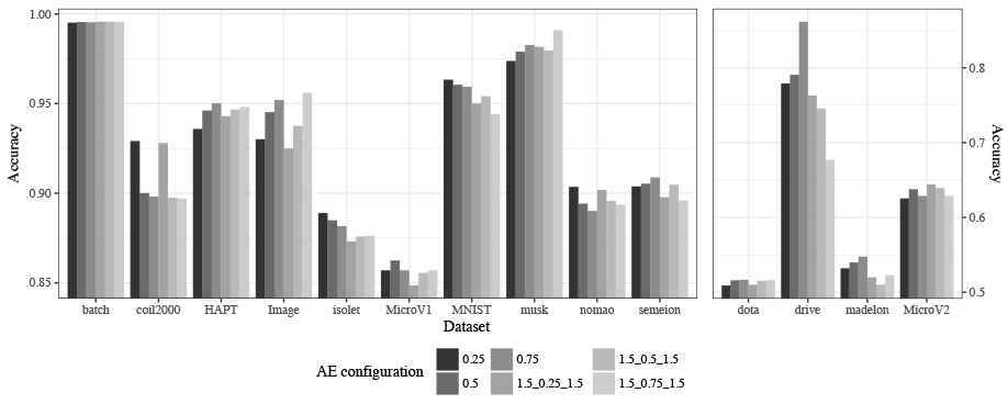
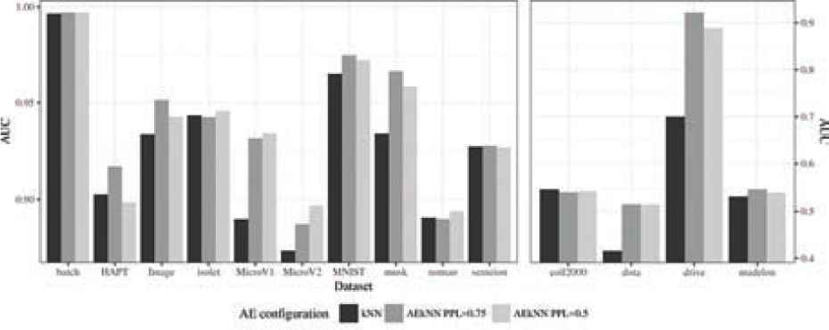
The results produced by the different configurations considered are presented grouped by metric. Table 3 shows the results for Accuracy, Table 4 for F-Score, and Table 5 for AUC. These results are also graphically represented. Aiming to optimize the visualization, two plots with different scales have been produced for each metric. Figure 4 represents the results for Accuracy, Figure 5 for F-Score, and Figure 6 for AUC.
| Dataset | (0.25) | (0.5) | (0.75) | (1.5, 0.25, 1.5) | (1.5, 0.5, 1.5) | (1.5, 0.75, 1.5) |
|---|---|---|---|---|---|---|
| image | 0.930 | 0.945 | 0.952 | 0.925 | 0.938 | 0.956 |
| drive | 0.779 | 0.791 | 0.862 | 0.763 | 0.746 | 0.677 |
| coil2000 | 0.929 | 0.900 | 0.898 | 0.928 | 0.897 | 0.897 |
| dota | 0.509 | 0.516 | 0.517 | 0.510 | 0.515 | 0.516 |
| nomao | 0.904 | 0.894 | 0.890 | 0.902 | 0.896 | 0.894 |
| batch | 0.995 | 0.995 | 0.995 | 0.996 | 0.996 | 0.996 |
| musk | 0.974 | 0.979 | 0.983 | 0.982 | 0.980 | 0.991 |
| semeion | 0.904 | 0.905 | 0.909 | 0.898 | 0.905 | 0.896 |
| madelon | 0.532 | 0.540 | 0.547 | 0.520 | 0.510 | 0.523 |
| hapt | 0.936 | 0.946 | 0.950 | 0.943 | 0.947 | 0.948 |
| isolet | 0.889 | 0.885 | 0.882 | 0.873 | 0.876 | 0.876 |
| mnist | 0.963 | 0.960 | 0.959 | 0.950 | 0.954 | 0.944 |
| microv1 | 0.857 | 0.863 | 0.857 | 0.849 | 0.856 | 0.857 |
| microv2 | 0.625 | 0.638 | 0.629 | 0.644 | 0.639 | 0.629 |
Bold values represent the best result in each case for different datasets and metrics.
Accuracy classification results for test data.
| Dataset | (0.25) | (0.5) | (0.75) | (1.5, 0.25, 1.5) | (1.5, 0.5, 1.5) | (1.5, 0.75, 1.5) |
|---|---|---|---|---|---|---|
| image | 0.930 | 0.945 | 0.952 | 0.925 | 0.938 | 0.956 |
| drive | 0.782 | 0.796 | 0.863 | 0.772 | 0.746 | 0.683 |
| coil2000 | 0.963 | 0.947 | 0.946 | 0.962 | 0.946 | 0.945 |
| dota | 0.481 | 0.487 | 0.486 | 0.481 | 0.488 | 0.485 |
| nomao | 0.905 | 0.897 | 0.893 | 0.904 | 0.898 | 0.897 |
| batch | 0.995 | 0.995 | 0.995 | 0.995 | 0.995 | 0.995 |
| musk | 0.984 | 0.988 | 0.990 | 0.989 | 0.988 | 0.995 |
| semeion | 0.905 | 0.906 | 0.910 | 0.899 | 0.905 | 0.896 |
| madelon | 0.549 | 0.542 | 0.567 | 0.531 | 0.501 | 0.529 |
| hapt | 0.818 | 0.829 | 0.842 | 0.833 | 0.839 | 0.837 |
| isolet | 0.890 | 0.887 | 0.883 | 0.875 | 0.878 | 0.878 |
| mnist | 0.963 | 0.960 | 0.959 | 0.950 | 0.954 | 0.944 |
| microv1 | 0.868 | 0.872 | 0.867 | 0.861 | 0.867 | 0.868 |
| microv2 | 0.619 | 0.636 | 0.625 | 0.641 | 0.643 | 0.628 |
Bold values represent the best result in each case for different datasets and metrics.
F-score classification results for test data.
| Dataset | (0.25) | (0.5) | (0.75) | (1.5, 0.25, 1.5) | (1.5, 0.5, 1.5) | (1.5, 0.75, 1.5) |
|---|---|---|---|---|---|---|
| image | 0.932 | 0.943 | 0.951 | 0.923 | 0.936 | 0.956 |
| drive | 0.881 | 0.889 | 0.922 | 0.875 | 0.850 | 0.826 |
| coil2000 | 0.526 | 0.543 | 0.541 | 0.526 | 0.538 | 0.539 |
| dota | 0.508 | 0.514 | 0.515 | 0.508 | 0.514 | 0.514 |
| nomao | 0.903 | 0.894 | 0.890 | 0.901 | 0.895 | 0.893 |
| batch | 0.997 | 0.997 | 0.997 | 0.997 | 0.997 | 0.997 |
| musk | 0.950 | 0.958 | 0.966 | 0.967 | 0.962 | 0.983 |
| semeion | 0.927 | 0.927 | 0.928 | 0.923 | 0.923 | 0.922 |
| madelon | 0.532 | 0.540 | 0.547 | 0.520 | 0.513 | 0.523 |
| hapt | 0.888 | 0.898 | 0.917 | 0.900 | 0.916 | 0.915 |
| isolet | 0.948 | 0.946 | 0.942 | 0.938 | 0.941 | 0.940 |
| mnist | 0.974 | 0.972 | 0.975 | 0.965 | 0.968 | 0.958 |
| microv1 | 0.928 | 0.934 | 0.931 | 0.932 | 0.927 | 0.927 |
| microv2 | 0.891 | 0.897 | 0.887 | 0.897 | 0.890 | 0.885 |
Bold values represent the best result in each case for different datasets and metrics.
Area under the ROC curve (AUC) classification results for test data.
Accuracy classification results for test data.
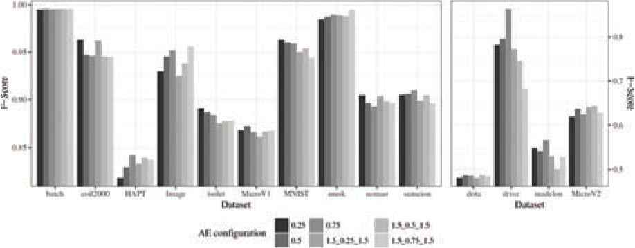
F-score classification results for test data.
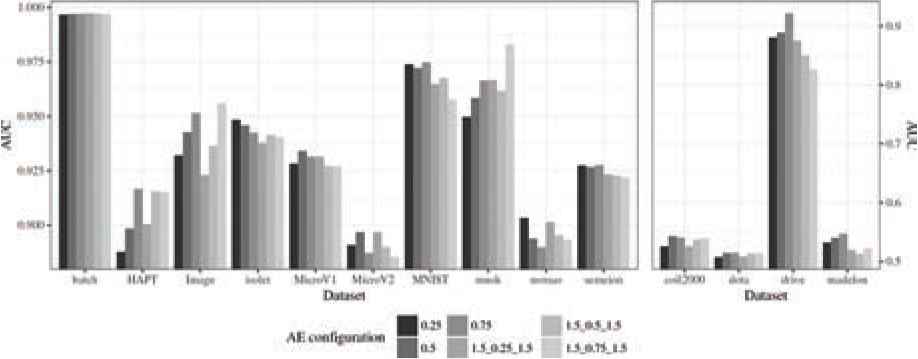
Area under the ROC curve (AUC) classification results for test data.
The results presented in Table 3 and in Figure 4 show the Accuracy obtained for AEkNN with different PPL values. These results indicate that there is no one configuration that works best for all datasets. The configurations with 3 hidden layers obtain the best results in 4 out of 14 datasets, whereas the configurations with 1 hidden layer win in 10 out of 14 datasets. This trend can also be seen in the graphs.
Table 4 and Figure 5 show the F-Score obtained by AEkNN with different PPL values. The values indicate that the configurations with one single hidden layer obtain better results in 11 out of 14 datasets. The configuration with PPL = (0.25) and with PPL = (0.75) are the ones winning more times (5). The version with PPL = (0.25) shows disparate results, the best values for some cases and bad results for other cases, for example, with hapt, image, or microv2. Although the version with PPL = (0.75) wins the same number of times, its results are more balanced.
In Table 5 the results for AUC obtained with AEkNN can be seen. Figure 6 represents those results. For this metric, it can be appreciated that single hidden layer structures work better, obtaining top results in 12 out of 14 datasets. However, a configuration that works best for all cases has not been found.
Summarizing, the results presented above show the metrics obtained for AEkNN with different PPL values. These results show some variability. The PPL value that obtains the best performance cannot be determined exactly, since for each dataset there is a setting that works best. However, some initial trends can be drawn:
Single-layer configuration: Better results than configurations with three hidden layers. For Accuracy and F-Score 71% of the best results are with 1 hidden layer, and for AUC this rises to 85%.
Configurations with PPL = (0.75): For AUC 50% of the best results are with this configuration. Their values are close to the best in most cases.
Configurations with PPL = (0.5): 29% of the best results are obtained with this parametrization if AUC is considered. In general, results are good in many cases.
Other configurations: Some good results but at other times they are far from the best values.
Once the results have been obtained, it is necessary to determine if there are statistically significant differences for each one of them in order to select the best configuration. To do this, the Friedman test [65] will be applied. Average ranks obtained by applying the Friedman test for Accuracy, F-Score, and AUC measures are shown in Table 6. In addition, Table 7 shows the different p-values obtained by the Friedman test.
| Accuracy | F-Score | AUC | |||
|---|---|---|---|---|---|
| PPL | Ranking | PPL | Ranking | PPL | Ranking |
| (0.75) | 2.679 | (0.5) | 2.923 | (0.75) | 2.357 |
| (0.5) | 2.857 | (0.75) | 3.000 | (0.5) | 2.786 |
| (0.25) | 3.714 | (0.25) | 3.429 | (1.5, 0.25, 1.5) | 3.786 |
| (1.5, 0.75, 1.5) | 3.821 | (1.5, 0.5, 1.5) | 3.500 | (0.25) | 3.857 |
| (1.5, 0.5, 1.5) | 3.892 | (1.5, 0.25, 1.5) | 4.071 | (1.5, 0.5, 1.5) | 4.000 |
| (1.5, 0.25, 1.5) | 4.036 | (1.5, 0.75, 1.5) | 4.071 | (1.5, 0.75, 1.5) | 4.214 |
PPl, percentage of elements per layer; AUC, area under the ROC curve.
Average rankings of the different PPL values by measure.
| Accuracy | F-Score | AUC |
|---|---|---|
| 0.236 | 0.423 | 0.049 |
AUC, area under the ROC curve.
Results of Friedman’s test (p-values).
As can be observed in Table 7, for AUC (which is considered a stronger performance metric) there are statistically significant differences between the considered PPL values if we set the p-value threshold to the usual range [0.05, 0.1]. However, for Accuracy and F-Score there are no statistically significant differences. In addition, in the rankings obtained, it can be seen that there are two specific configurations that offer better results than the remaining ones. In the three rankings presented, the results with PPL = (0.75) and PPL = (0.5) appear first, clearly highlighted with respect to the other values. Therefore, it is considered that these two configurations are the best ones. Thus, the results of AEkNN with both configurations will be compared against the kNN algorithm.
5.3. AEkNN versus kNN
This second part is focused on determining whether the results obtained with the proposed algorithm, AEkNN, improve those obtained with the kNN algorithm. To do so, a comparison will be made between the results obtained with AEkNN, using the values of the PPL parameter selected in the previous section, and the results obtained with kNN algorithm on the same datasets.
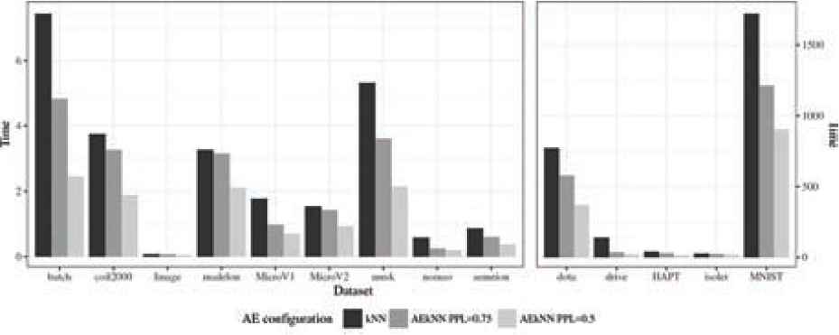
First, Table 8 shows the results for each one of the datasets and considered measures, including running time. The results for both algorithms are presented jointly, and the best ones are highlighted in bold. Two plots have been generated for each metric, aiming to optimize data visualization, as in the previous phase, since the range of results was very broad. Figure 7 represents the results for Accuracy, Figure 8 for F-Score, Figure 9 for AUC, and Figure 10 for runtime.
| Accuracy | F-Score | AUC | Time (Seconds) | |||||||||
|---|---|---|---|---|---|---|---|---|---|---|---|---|
| kNN | AEkNN | kNN | AEkNN | kNN | AEkNN | kNN | AEkNN | |||||
| Dataset | (0.75) | (0.5) | (0.75) | (0.5) | (0.75) | (0.5) | (0.75) | (0.5) | ||||
| image | 0.937 | 0.952 | 0.945 | 0.937 | 0.952 | 0.945 | 0.934 | 0.951 | 0.943 | 0.074 | 0.073 | 0.052 |
| drive | 0.691 | 0.862 | 0.791 | 0.615 | 0.863 | 0.796 | 0.700 | 0.922 | 0.889 | 139.623 | 36.977 | 20.479 |
| coil2000 | 0.897 | 0.898 | 0.900 | 0.945 | 0.946 | 0.947 | 0.547 | 0.541 | 0.543 | 3.753 | 3.262 | 1.886 |
| dota | 0.507 | 0.517 | 0.516 | 0.479 | 0.486 | 0.487 | 0.416 | 0.515 | 0.514 | 772.219 | 578.437 | 370.599 |
| nomao | 0.891 | 0.890 | 0.894 | 0.892 | 0.893 | 0.897 | 0.891 | 0.890 | 0.894 | 0.582 | 0.252 | 0.200 |
| batch | 0.995 | 0.995 | 0.995 | 0.995 | 0.995 | 0.995 | 0.996 | 0.997 | 0.997 | 7.433 | 4.829 | 2.459 |
| musk | 0.956 | 0.983 | 0.979 | 0.974 | 0.990 | 0.988 | 0.934 | 0.966 | 0.958 | 5.317 | 3.613 | 2.144 |
| semeion | 0.908 | 0.909 | 0.905 | 0.910 | 0.910 | 0.906 | 0.927 | 0.928 | 0.927 | 0.865 | 0.601 | 0.381 |
| madelon | 0.531 | 0.547 | 0.540 | 0.549 | 0.567 | 0.542 | 0.532 | 0.547 | 0.540 | 3.267 | 3.150 | 2.109 |
| hapt | 0.951 | 0.950 | 0.946 | 0.842 | 0.842 | 0.829 | 0.903 | 0.917 | 0.898 | 41.673 | 30.625 | 16.365 |
| isolet | 0.872 | 0.882 | 0.885 | 0.874 | 0.883 | 0.887 | 0.943 | 0.942 | 0.946 | 27.563 | 24.748 | 19.538 |
| mnist | 0.947 | 0.959 | 0.960 | 0.946 | 0.959 | 0.960 | 0.965 | 0.975 | 0.972 | 1720.547 | 1213.168 | 904.223 |
| microv1 | 0.800 | 0.857 | 0.863 | 0.806 | 0.867 | 0.872 | 0.890 | 0.931 | 0.934 | 1.776 | 0.977 | 0.709 |
| microv2 | 0.607 | 0.629 | 0.638 | 0.603 | 0.625 | 0.636 | 0.873 | 0.887 | 0.897 | 1.542 | 1.425 | 0.933 |
PPL, percentage of elements per layer; kNN, k-nearest neighbors; AUC, area under the ROC curve.
Bold values represent the best result in each case for different datasets and metrics.
Classification results of AEkNN (with different PPL) and kNN algorithm for test data.
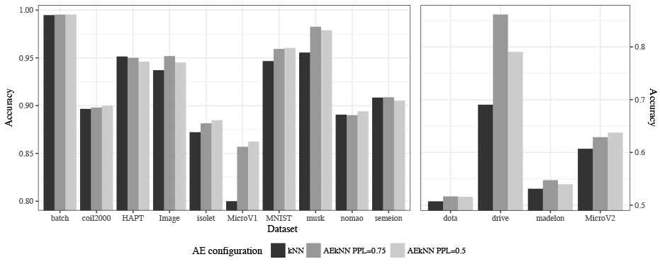
Accuracy results for test data.
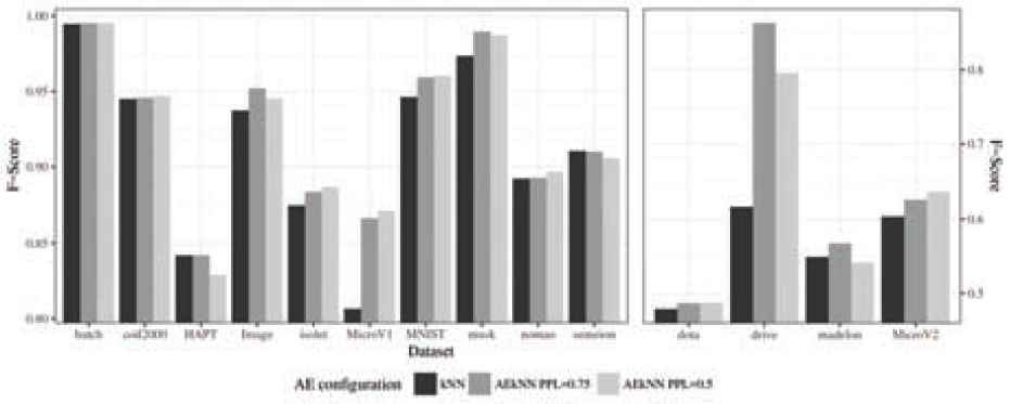
F-score results for test data.
Area under the ROC curve (AUC) results for test data.
Time results for test data.
The results shown in Table 8 indicate that AEkNN works better than kNN for most datasets considering Accuracy. On the one hand, the version of AEkNN with PPL = (0.75) improves kNN in 11 out of 14 cases, obtaining the best overall results in 6 of them. On the other hand, the version of AEkNN with PPL = (0.5) obtains better results than kNN in 11 out of 14 cases, and is the best configuration in 6 of them. In addition, kNN only obtains one best result. Figure 7 confirms this trend. It can be observed that the right bars, where AEkNN results are represented, are higher in most datasets.
Analyzing the data corresponding to the metric F-Score, presented in Table 8, it can be observed that AEkNN produces an overall improvement over kNN. The AEkNN version with PPL = (0.75) improves kNN in 11 out of 14 cases, obtaining the best overall results in 5 of them. The version of AEkNN with PPL = (0.5) obtains better results than kNN in 10 out of 14 cases, and is the best configuration in 7 of them. kNN does not obtain any best result. How the results of the versions corresponding to AEkNN produce higher values than those corresponding to kNN can be seen in Figure 8.
The data related to AUC, presented in Table 8, also show that AEkNN works better than kNN. In this case, the two versions of AEkNN improve kNN in 11 out of 14 cases each one, obtaining the best results in 13 out of 14 cases. Figure 9 shows that the trend is increasing towards the versions of the new algorithm. kNN only obtains one best result, specifically with the coil2000 dataset, which may be due to the low number of features in this dataset. Nonetheless, AEkNN performs better than kNN in the rest of metrics for coil2000 dataset.
The running times for both algorithms are presented in Table 8 and Figure 10. As can be seen, the configuration that takes less time to classify is the one corresponding to AEkNN with PPL = (0.5), obtaining the lowest value for all datasets. This is due to the higher compression of the data achieved by this configuration. In the same way, AEkNN with PPL = (0.75) obtains better results than the algorithm kNN in all cases.
Summarizing, the following conclusions can be drawn from the previous analysis:
Accuracy: 93% of the best results are obtained with AEkNN. Both AEkNN configurations considered behave in a similar way. kNN only improves in one case.
F-Score: AEkNN obtains the best results in 100% of the cases. The configurations used have a similar performance. kNN ties with AEkNN in three cases.
AUC: The best results are obtained with AEkNN in 93% of the datasets. The configuration with PPL = (0.75) stands out, achieving the best results in 64% of cases. kNN improves in one case.
Time: Both AEkNN configurations improve kNN in 100% of cases. AEkNN with PPL = (0.5) obtains the best results in all cases.
To sum up, AEkNN performs a transformation of the input space to reduce dimensionality. In spite of this, the quality of the results in terms of classification performance are better than those of kNN in most cases. In addition, in terms of classification time, it can be noted how AEkNN, with higher compression of information, significantly reduces the time spent on classification, without having a negative impact on the other measures.
To determine if there are statistically significant differences between the obtained results, the proper statistical test has been conducted. For this purpose, the Wilcoxon test will be performed, comparing each version of AEkNN against the results of the classical kNN algorithm. In Table 9, the results obtained for Wilcoxon tests are shown.
| Accuracy | F-Score | AUC | Time | |
|---|---|---|---|---|
| AEkNN with PPL = (0.75) | 0.0017 | 0.0003 | 0.0085 | 0.0002 |
| AEkNN with PPL = (0.5) | 0.0023 | 0.0245 | 0.0107 | 0.0001 |
kNN, k-nearest neighbor; AUC, area under the ROC curve, PPL, percentage of elements per layer.
Result of Wilcoxon’s test (p-values) comparing kNN versus AEkNN.
As can be seen the p-values are rather low, so statistically significant differences between the two AEkNN versions and the original kNN algorithm in all considered measures exist can be concluded, considering the p-value threshold within the usual [0.05, 0.1] range. On the one hand, taking into account Accuracy, F-Score, and AUC, the configuration with best results is that with 75% of feature reduction. Therefore, this is the optimal solution from the point of view of predictive performance. The reason for this might be that there is less compression of the data, therefore, there is less loss of information compared to the other considered configuration (50%). On the other hand, considering running time, the configuration with best results is that with 50% of feature reduction. It is not surprising that having fewer features allows to compute distances in less time.
5.4. AEkNN vs PCA/LDA
The objective of this third part is to assess the competitiveness of AEkNN against traditional dimensionality reduction algorithms. Specifically, the algorithms used will be PCA [42] and LDA [70], since they are traditional algorithms that offer good results in this task [71]. To do so, a comparison will be made between the results obtained with AEkNN, using the values of the PPL parameter selected in Section 5.3, and the results obtained with PCA and LDA algorithm on the same datasets. It is important to note that the number of features selected with these methods will be the same as with the AEkNN algorithm, so there are two executions for each algorithm.
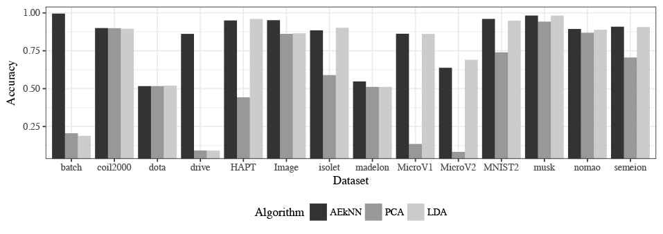
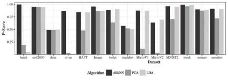
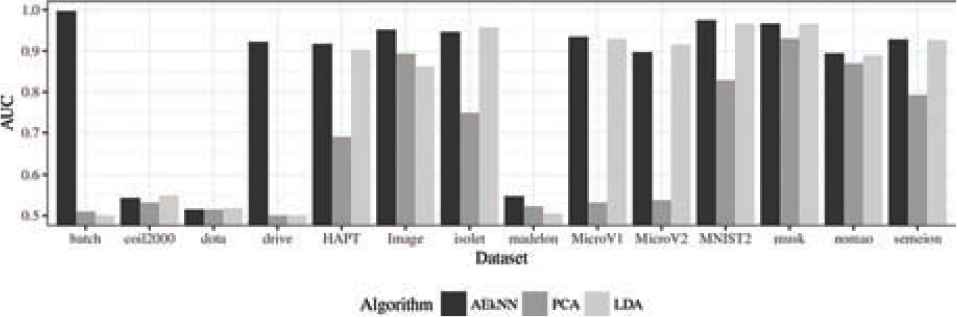
First, Table 10 shows the results for each one of the datasets and considered measures. The results for the three algorithms are presented jointly, and the best ones are highlighted in bold. One plot have been generated for each metric aiming to optimize data visualization. In this case, the graphs represent the best value of the two configurations for each algorithm in order to better visualize the differences between the three methods. Figure 11 represents the results for Accuracy, Figure 12 for F-Score, and Figure 13 for AUC.
| Accuracy | F-Score | AUC | |||||||||||||||||
|---|---|---|---|---|---|---|---|---|---|---|---|---|---|---|---|---|---|---|---|
| AEkNN | PCA | LDA | AEkNN | PCA | LDA | AEkNN | PCA | LDA | |||||||||||
| Dataset | (0.75) | (0.5) | (0.75) | (0.5) | (0.75) | (0.5) | (0.75) | (0.5) | (0.75) | (0.5) | (0.75) | (0.5) | (0.75) | (0.5) | (0.75) | (0.5) | (0.75) | (0.5) | |
| image | 0.952 | 0.945 | 0.563 | 0.862 | 0.676 | 0.866 | 0.952 | 0.945 | 0.580 | 0.867 | 0.672 | 0.866 | 0.951 | 0.943 | 0.734 | 0.893 | 0.780 | 0.862 | |
| drive | 0.862 | 0.791 | 0.091 | 0.092 | 0.091 | 0.091 | 0.863 | 0.796 | 0.023 | 0.030 | 0.015 | 0.015 | 0.922 | 0.889 | 0.500 | 0.491 | 0.500 | 0.500 | |
| coil2000 | 0.898 | 0.900 | 0.825 | 0.899 | 0.895 | 0.895 | 0.946 | 0.947 | 0.861 | 0.946 | 0.944 | 0.944 | 0.541 | 0.543 | 0.523 | 0.532 | 0.545 | 0.549 | |
| dota | 0.517 | 0.516 | 0.514 | 0.517 | 0.519 | 0.520 | 0.486 | 0.487 | 0.486 | 0.486 | 0.489 | 0.493 | 0.515 | 0.514 | 0.513 | 0.515 | 0.517 | 0.519 | |
| nomao | 0.890 | 0.894 | 0.798 | 0.869 | 0.818 | 0.889 | 0.893 | 0.897 | 0.821 | 0.871 | 0.851 | 0.891 | 0.890 | 0.894 | 0.797 | 0.869 | 0.817 | 0.889 | |
| batch | 0.995 | 0.995 | 0.195 | 0.206 | 0.189 | 0.152 | 0.995 | 0.995 | 0.176 | 0.190 | 0.053 | 0.044 | 0.997 | 0.997 | 0.502 | 0.510 | 0.500 | 0.500 | |
| musk | 0.983 | 0.979 | 0.942 | 0.931 | 0.982 | 0.982 | 0.990 | 0.988 | 0.962 | 0.945 | 0.989 | 0.989 | 0.966 | 0.958 | 0.912 | 0.930 | 0.965 | 0.965 | |
| semeion | 0.909 | 0.905 | 0.598 | 0.706 | 0.907 | 0.890 | 0.910 | 0.906 | 0.624 | 0.718 | 0.906 | 0.893 | 0.928 | 0.927 | 0.732 | 0.792 | 0.926 | 0.913 | |
| madelon | 0.547 | 0.540 | 0.506 | 0.511 | 0.501 | 0.512 | 0.567 | 0.542 | 0.519 | 0.503 | 0.503 | 0.491 | 0.547 | 0.540 | 0.523 | 0.510 | 0.505 | 0.505 | |
| hapt | 0.950 | 0.946 | 0.179 | 0.443 | 0.959 | 0.960 | 0.842 | 0.829 | 0.180 | 0.478 | 0.841 | 0.841 | 0.917 | 0.898 | 0.553 | 0.690 | 0.903 | 0.899 | |
| isolet | 0.882 | 0.885 | 0.424 | 0.590 | 0.886 | 0.902 | 0.883 | 0.887 | 0.504 | 0.638 | 0.888 | 0.903 | 0.942 | 0.946 | 0.660 | 0.748 | 0.951 | 0.957 | |
| mnist | 0.959 | 0.960 | 0.740 | 0.640 | 0.949 | 0.943 | 0.959 | 0.960 | 0.704 | 0.704 | 0.949 | 0.943 | 0.975 | 0.972 | 0.828 | 0.798 | 0.966 | 0.954 | |
| microv1 | 0.857 | 0.863 | 0.135 | 0.135 | 0.818 | 0.861 | 0.867 | 0.872 | 0.116 | 0.116 | 0.823 | 0.871 | 0.931 | 0.934 | 0.532 | 0.532 | 0.898 | 0.929 | |
| microv2 | 0.629 | 0.638 | 0.058 | 0.082 | 0.649 | 0.690 | 0.625 | 0.636 | 0.005 | 0.037 | 0.644 | 0.695 | 0.887 | 0.897 | 0.500 | 0.537 | 0.891 | 0.916 | |
kNN, k-nearest neighbor; AUC, area under the ROC curve, PPL, percentage of elements per layer; LDA, linear discriminant analysis; PCA, principal components analysis.
Bold values represent the best result in each case for different datasets and metrics.
Accuracy, F-Sscore, and AUC classification results of AEkNN (with different PPL), LDA, and PCA for test data.
Accuracy results for test data.
F-score results for test data.
Area under the ROC curve (AUC) results for test data.
The results shown in Table 10 indicate that AEkNN works better than PCA and LDA for most datasets considering Accuracy. On the one hand, the version of AEkNN with PPL = (0.75) improves PCA in 12 out of 14 cases and LDA in 9 out of 14 cases, obtaining the best overall results in 7 of them. On the other hand, the version of AEkNN with PPL = (0.5) obtains better results than PCA in 13 out of 14 cases and LDA in 8 out of 14 cases, and is the best configuration in 4 of them. In addition, LDA only obtains the best result in 4 cases. Figure 11 confirms this trend. It can be observed that the bars, where AEkNN results are represented, are higher in most datasets.
Analyzing the data corresponding to the metric F-Score, presented in Table 10, it can be observed that AEkNN produces an overall improvement over PCA and LDA. The AEkNN version with PPL = (0.75) improves PCA in 12 out of 14 cases and LDA in 10 out of 14 cases, obtaining the best overall results in 6 of them. The version of AEkNN with PPL = (0.5) obtains better results than PCA in all cases and LDA in 8 out of 14 cases, and is the best configuration in 4 of them. PCA does not obtain any best result and LDA obtains the best result in 4 cases. How the results of the versions corresponding to AEkNN show values higher than those corresponding to kNN can be seen in Figure 12.
The data related to AUC, presented in Table 10, also show that AEkNN works better than PCA and LDA. The AEkNN version with PPL = (0.75) improves PCA in 13 out of 14 cases and LDA in 10 out of 14 cases, obtaining the best overall results in 7 of them. The version of AEkNN with PPL = (0.5) obtains better results than PCA in 13 out of 14 cases and LDA in 8 out of 14 cases, and is the best configuration in 4 of them. LDA only obtains the best result in 4 cases. Figure 13 confirms this trend.
Summarizing, these results show some trends that are listed below:
Accuracy: 71% of the best results are obtained by AEkNN. LDA improves AEkNN in 29% of the cases. AEkNN is always close to the best result. PCA does not surpass AEkNN in any case.
F-Score: AEkNN obtains the best results in 79% of the cases. LDA generates better performance in 21% of the cases. AEkNN always improves PCA.
AUC: The best results are obtained by AEkNN in 71% of the datasets. LDA achieves the best results in 29% of cases. PCA does not improve in any dataset.
The quality of the results with AEkNN in terms of classification performance are better than those of PCA and LDA in most cases. This means that the high-level features obtained by the AEkNN algorithm provides more relevant information than those obtained by the PCA and LDA algorithms.
Previously, the data obtained in the experimentation have been presented and a comparison between them is made. However, it is necessary to verify whether there are significant differences between the data corresponding to the different algorithms. To do so, the Friedman test [65] will be applied. Average ranks obtained by applying the Friedman test for Accuracy, F-Score, and AUC measures are shown in Table 11. In addition, Table 12 shows the different p-values obtained by the Friedman test.
| Accuracy | F-Score | AUC | |||
|---|---|---|---|---|---|
| Algorithm | Ranking | Algorithm | Ranking | Algorithm | Ranking |
| AEkNN PPL = 0.75 | 2.286 | AEkNN PPL = 0.75 | 2.143 | AEkNN PPL = 0.75 | 1.929 |
| AEkNN PPL = 0.5 | 2.357 | AEkNN PPL = 0.5 | 2.214 | AEkNN PPL = 0.5 | 2.500 |
| LDA PPL = 0.5 | 3.000 | LDA PPL = 0.75 | 3.429 | LDA PPL = 0.5 | 2.929 |
| LDA PPL = 0.75 | 3.571 | LDA PPL = 0.5 | 3.429 | LDA PPL = 0.75 | 3.500 |
| PCA PPL = 0.5 | 4.321 | PCA PPL = 0.5 | 4.429 | PCA PPL = 0.5 | 4.679 |
| PCA PPL = 0.75 | 5.464 | PCA PPL = 0.75 | 5.357 | PCA PPL = 0.75 | 5.464 |
kNN, k-nearest neighbor; AUC, area under the ROC curve, PPL, percentage of elements per layer; LDA, linear discriminant analysis; PCA, principal components analysis.
Average rankings of the different dimensionality reduction algorithms by measure.
| Accuracy | F-Score | AUC |
|---|---|---|
| 1.266e-05 | 7.832e-06 | 7.913e-07 |
AUC, area under the ROC curve.
Results of Friedman’s test (p-values).
As can be observed in Table 12, for Accuracy, F-Score, and AUC there are statistically significant differences between the different PPL values if we set the p-value threshold to the usual range [0.05, 0.1]. It can be seen that AEkNN with PPL = (0.75) offer better results than the remaining ones. In the three rankings presented, the AEkNN configurations with PPL = (0.75) and PPL = (0.5) appear first, clearly highlighted with respect to the other values. Therefore, it is considered that AEkNN obtains better predictive performance, since the reduction of dimensionality generates more significant features.
5.5. General Guidelines on the Use of AEkNN
AEkNN could be considered as a robust algorithm on the basis of the previous analysis. The experimental study demonstrates that it has good performance with the two PPL considered values. From the conducted experimentation some guidelines can also be extracted:
When working with very high-dimensional datasets, it is recommended to use AEkNN with the PPL = (0.5) configuration. In this study, this configuration has obtained the best results for datasets containing more than 600 features. The reason is that the input data has a larger number of features and allows a greater reduction without losing relevant information. Therefore, AEkNN can compress more in these cases.
When using binary datasets with a lower dimensionality, the AEkNN algorithm with the PPL = (0.5) configuration continues to be the best choice. In our experience, this configuration has shown to work better for binary datasets with a number of features around 100. In these cases, the compression may be higher since it is easier to discriminate by class.
For all other datasets, the choice of configuration for AEkNN depends on the indicator to be enhanced. On the one hand, if the goal is to achieve the best possible predictive performance, the configuration with PPL = (0.75) must be chosen. In these cases, AEkNN needs to generate more features. On the other hand, when the interest is to optimize the running time, while maintaining improvements in predictive performance with respect to kNN, the configuration with PPL = (0.5) is the best selection. The reason is in the higher compression of the data. AEkNN needs less time to classify lower-dimensional data.
Summarizing, the configuration of AEkNN must be adapted to the data traits to obtain optimal results. For this, a series of tips have been established.
5.6. AEkNN Application to Real Cases
The main objective of this section is to present the results of applying AEkNN to real cases. To do this, two datasets with a large number of features have been used:
Arcene: This dataset belongs to the medical field. The objective is to derive patterns corresponding to patients with cancer. The dataset have 10000 features and 900 instances [61].
Gisette: It is an image recognition dataset. It consists in separating the digits 4 and 9. This set contains 5,000 characteristics and 13500 examples [61].
Following the recommendations established in the Section 5.5, the configuration of AEkNN used is with PPL = (0.5), since both are datasets with a very high dimensionality. Next, the results obtained with AEkNN and kNN are shown for both datasets.
Table 13 shows the behavior of AEkNN when applying it to real cases. In both datasets the results obtained with AEkNN obtain better performance than those obtained with the classic kNN algorithm. For Arcene, the improvement of AEkNN with respect to kNN in the three metrics considered is higher than 4% and for Gisette it is higher than 2%. In terms of execution time, the reduction obtained is very significant in excess of 50% in both cases.
| Accuracy | F-Score | AUC | Time (Seconds) | |||||||||
|---|---|---|---|---|---|---|---|---|---|---|---|---|
| kNN | AEkNN | % | kNN | AEkNN | % | kNN | AEkNN | % | kNN | AEkNN | % | |
| arcene | 0.682 | 0.714 | 4.692 | 0.679 | 0.712 | 4.861 | 0.689 | 0.722 | 4.789 | 34.582 | 11.834 | 65.779 |
| gisette | 0.823 | 0.841 | 2.187 | 0.824 | 0.844 | 2.427 | 0.823 | 0.849 | 3.159 | 256.231 | 119.723 | 53.275 |
AUC, area under the ROC curve; kNN, k-nearest neighbor.
AEkNN versus kNN results in real cases and %percent improvement.
In summary, the analysis of the application of AEkNN to real cases shows the improvements obtained with the method proposed in this work. Additionally, it provides the reader with an application example for other similar problems.
6. CONCLUDING REMARKS
In this paper, a new classification algorithm called AEkNN has been proposed. This algorithm is based on kNN but aims to mitigate the problem that arises when working with high-dimensional data. To do so, AEkNN internally incorporates a model-building phase aimed at achieving a reduction of the feature space, using AEs for this purpose. The main reason that has led to the design of AEkNN are the good results that have been obtained by AEs when they are used to generate higher-level features. AEkNN relies on an AE to extract a reduced representation of a higher level that replaces the original data.
In order to determine if the proposed algorithm has better behavior than the kNN algorithm, an experimentation process has been followed. Firstly, the analysis of different AE architectures have allowed to determine which structure works better. In this sense, single-layer configurations obtain the best performance in more than 71% of the datasets considering the different metrics.
Furthermore, in the second part of the conducted experimentation, AEkNN with the best configurations have been compared with classical kNN. As has been stated, the results of AEkNN improve those obtained by kNN in all metrics. Specifically, AEkNN obtains the best performance in more than 93% for all metrics. In addition, AEkNN offers a considerable improvement with respect to the time invested in the classification. In this sense, AEkNN works better than kNN in 100% of the datasets.
In addition, a comparison has been made with other traditional methods applied to this problem, in order to verify that the AEkNN algorithm improves behavior when carrying out the dimensionality reduction task. For this, AEkNN has been compared with LDA and PCA. The results show that the proposed AEkNN algorithm improves performance in classification for most of the dataset used. In more detail, AEkNN always improves PCA and exceeds at least 71% of the dataset to LDA, according to the considered metrics. This occurs because the features generated with the proposed algorithm are more significant and provide more relevant information to the classification using distance-based algorithms.
Finally, AEkNN has been applied to solve real problems. Given two datasets corresponding to different fields, AEkNN has been applied following the guidelines set out in the article. This analysis shows clear improvements in terms of predictive performance and execution time with respect to the classic kNN algorithm. It is important to highlight that all the conclusions reached throughout the experimentation have been confirmed by statistical tests where significant differences are obtained.
In conclusion, AEkNN is able to reduce the adverse effects of high-dimensional data while performing instance-based classification, improving both running time and classification performance. This paper shows that the use of AEs can be helpful to solve this kind of obstacle, opening up new possibilities of future work in which they are applied to help solve similar problems presented by other traditional models.
ACKNOWLEDGMENT
The work of F. Pulgar was supported by the Spanish Ministry of Education under the FPU National Program (Ref. FPU16/00324). This work was partially supported by the Spanish Ministry of Science and Technology under project TIN2015-68454-R.
REFERENCES
Cite this article
TY  - JOUR
AU  - Francisco J. Pulgar
AU  - Francisco Charte
AU  - Antonio J. Rivera
AU  - María J. del Jesus
PY  - 2019
DA  - 2019/02/28
TI  - AEkNN: An AutoEncoder kNN-Based Classifier With Built-in Dimensionality Reduction
JO  - International Journal of Computational Intelligence Systems
SP  - 436
EP  - 452
VL  - 12
IS  - 1
SN  - 1875-6883
UR  - https://doi.org/10.2991/ijcis.2018.125905686
DO  - 10.2991/ijcis.2018.125905686
ID  - Pulgar2019
ER  -